Chapter 1: Thinking Multiplicatively
1.1 Introduction
As explained in the Introduction, the aim behind this website is to invest in teaching each BIG Idea until it is really well understood – to the point where the uses of it are essentially trivial. For this to work, you can’t rush the BIG Idea itself – learners need time to make sense of it and see it from multiple angles.
Abraham Lincoln is supposed to have said, “Give me six hours to chop down a tree and I will spend the first four sharpening the axe” (Figure 1.1).
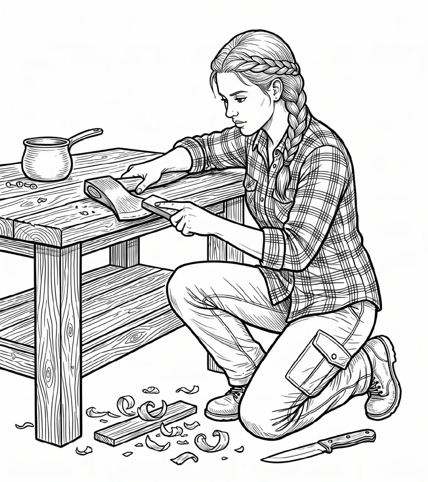
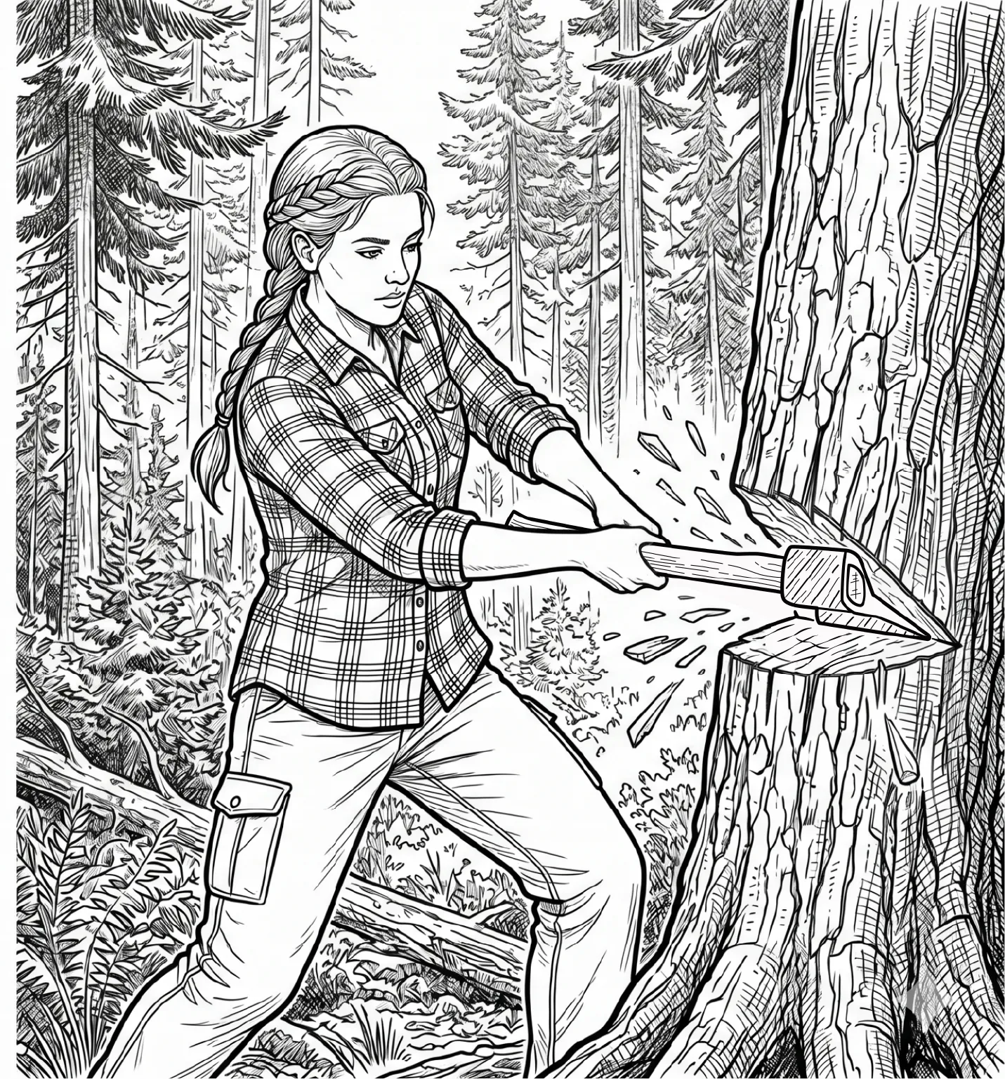
If you came along after three hours to see how he was getting on with his tree felling, progress would seem very disappointing – he hasn’t even started yet! This looks like procrastination, or lack of confidence to get moving – he seems stuck in his preparation. By contrast, if you came along after five hours, you would be astonished at how quickly the tree was coming down. You might pause to watch his technique with the axe. But when you try to imitate the swing yourself later, on your own tree, with your own blunt axe, you will wonder what you are doing wrong. The key to his success is not apparent during the actual cutting down, but is hidden within the lengthy preparation of the axe.
I think something like this often happens when one teacher observes another teacher’s lesson. If learning is going well, it is often due to things the teacher did before, rather than during, the observed lesson – it is how the learners had been previously prepared. Investing time in building solid foundations means subsequent learning is much more likely to go smoothly, make sense and be memorable and satisfying, with less stress. But you do not get these benefits without committing to the preparatory work.
One of the most important BIG Ideas in school mathematics is around thinking multiplicatively. This is a key that unlocks a surprisingly large number of doors. In this chapter, we will see what thinking multiplicatively entails, why it is fundamentally difficult, and so requires concentrated attention, and what learners can go on to access once they have become confident with it.
1.2 Additive beginnings: the positive integers
The psychologist David Ausubel wrote that, “If I had to reduce all of educational psychology to just one principle, I would say this: The most important single factor influencing learning is what the learner already knows; ascertain this and teach [them] accordingly”.1 We always have to begin where learners are - there is no other option - and this is often not as multiplicative thinkers, but as additive thinkers. So, we will begin by contrasting multiplicative thinking with additive thinking.
How do you imagine learners would respond to this task?
How can we get from \(5\) to \(15\)?
\[ \begin{matrix} 5 & \fixedarrow{$ $} & 15 \\ \end{matrix} \]
There are many possible responses, but learners are very likely to say “Add \(10\)”:
\[ \begin{matrix} 5 & \fixedarrow{$+10$} & 15 \\ \end{matrix} \]
There is, of course, nothing wrong with this answer. They might even say “Add a one”, and if by this they mean a digit \(1\), in the \(10\)s column, then this is also correct. Writing a ‘\(1\)’ before the ‘\(5\)’ does indeed constitute ‘Adding \(10\)’ to the number in our base-\(10\) place value system.
Addition is the first of the mathematical operations learners encounter when very young and beginning to learn number names and the count sequence (\(0\)), \(1\), \(2\), \(3\), …., which is obviously the “Add \(1\)” sequence, starting at \(1\) (or \(0\)). Addition corresponds to accumulating more items, and these items might be identical, as in Figure 1.2, or varied, as in Figure 1.3.


If the items vary, they could do so, as here, by being the same dinosaur in various poses and orientations, or different dinosaurs, but still all dinosaurs.2
Alternatively, the things being counted could be more abstract symbols, as in Figure 1.4, which could be arranged in a more regular kind of way, as in Figure 1.5.


The dots might even be lined up neatly, as in Figure 1.6, which we could think of as being against a horizontal number line, where the marked numbers count the number of dots we have accumulated by that point, as in Figure 1.7.


Vertical number lines take advantage of gravity, if we imagine the objects being stacked, and then we have the convenience that ‘more’ corresponds to ‘higher’ amounts (Figure 1.8).

Vertical number lines also avoid the problem of having to remember the arbitrary convention that greater numbers are placed further to the right, and smaller numbers to the left. Many people get confused over which way is left or right, but no one forgets which way is up!3 Familiarity with both vertical and horizontal number lines is essential in school mathematics. Eventually, one of each of these will be put together to make Cartesian axes (Figure 1.9). I will discuss this much more in Chapter 4.

When the focus is on place value, it can be useful to visualise an ordered stack of number lines, one for each decade, which gives us a \(1\)-\(100\) (or \(0\)-\(99\)) square (Figure 1.10).45

Beginning with zero in the bottom left corner means that all the \(1\)-digit numbers are in the bottom row, and \(10\) is viewed as the zeroth member of the second (\(10\)s) decade, rather than the \(10\)th member of the first decade. Here, adding \(10\) corresponds to a vertical displacement one row up, and ‘higher’ numbers are higher up, as with a vertical number line.6
As soon as we have encountered the idea of adding \(1\), we are close to thinking about infinity, because what if we just carried on adding \(1\) and adding \(1\)? What could ever stop us from continuing? Both number lines and rectangles of numbers presuppose that there is no end to the positive integers, so this is a nice place to think about infinity, if learners don’t bring this up themselves, which I find they often do:7
Could there be a largest possible number?
In real life, things rarely continue for ever – there is always some limit – and learners often naturally carry over this belief into mathematics. But we can be quite sure there is no largest number, because we can always imagine adding \(1\) to any number we care to think of.
If we suppose we have found the largest possible number, then what will happen when we add \(1\) to it? We will get a larger number, which means we must have been wrong to suppose we had found the largest possible number! (This is a simple example of a proof by contradiction.)
Numbers go on forever, because you can always keep adding \(1\) to the latest number you have made, and get a larger number. Learners often worry that we might not have a name for every arbitrarily large number, but we could always just read out its digits. The longest word in the English language could not just be a random collection of letters; it would have to mean something, and someone would have had to have invented it. But with large numbers, it is not necessary that anyone has ever considered that number previously. Any specific, arbitrarily large number has almost certainly never been thought of by any person ever, which can be quite a mind-blowing thought.
1.3 Zero and the negative integers
As the inverse operation of addition, subtraction is generally harder to perform procedurally than the more basic process of addition. The standard written subtraction algorithms involve exchanging a \(10\) for ten \(1\)s, and so on (see Chapter 2). But conceptually, subtraction is no more difficult than addition. Subtraction involves removing objects, rather than accumulating them, and this can be represented by moving to the left (or down) rather than to the right (or up) on a number line.
However, there are some important differences. When we add positive integers together, we necessarily remain within the positive integers. (We say the positive integers are closed under addition.) But once we start subtracting positive integers, even if we do it from other positive integers, there is always the chance that we might try to subtract a number that is not smaller than the one we began with. And then we either have to say that calculations like that are impossible – not allowed – or else we have to expand what we count as a number, to include zero and the negative integers.
Saying that a calculation is impossible is not a silly or ignorant thing to do. It doesn’t necessarily mean you don’t know about some possible numbers that exist. Depending on the context, taking away more than you began with might make no sense at all. If five people go into a building and three people come out, can we conclude that there are two people left in the building? Yes, provided there were no other entries or exits – and provided we know the building was empty to begin with! But if we don’t know the building was empty at the start, then five people going into the building and six people coming out is not ridiculous at all, so long as there was at least one person in the building before we began counting. Even very young children appreciate this kind of thinking, for example when seeing magic tricks in which an object must have already been hidden somewhere beforehand. The calculation \(5 - 6\) might make sense or it might not, depending what there might be \(5\) or \(6\) of.
The \(0\)-\(99\) square representation in Figure 1.10 deliberately includes zero in the first box, rather than beginning at \(1\). Zero is the first difficult number that learners meet. Arbitrarily large positive integers can be big, but they are not conceptually difficult. We can always imagine getting there just by adding \(1\) a lot of times. But zero is difficult. Learners can’t look at zero of any number of objects, because there is nothing there to see. And the number \(1\) feels very much as though it ought to be the first number. (We can say that zero is the ‘zeroth’ number, if that helps.) Learners will often wonder if zero really is a number.8 How can ‘nothing’ be a number, when a number is ‘something’? This is an issue learners will get used to, but perhaps no one ever really gets past these philosophical difficulties over zero – it is certainly a very strange number, and we shouldn’t make our most thoughtful learners feel silly for thinking so.9
When counting backwards from \(10\), young learners may feel a desire to continue after they reach \(1\), such as by saying ‘Blast off’, if envisaging a rocket taking off. A young child counted backwards from \(10\), and reached zero, and then looked at the adult and said “Now what?” Since they asked the question, the adult chose to respond, “Negative \(1\), negative \(2\), negative \(3\), …” and the child joined in, and they carried on for a while. Subsequently, when counting backwards with other children, this child would continue past zero like this, after the other children had stopped. Although this child did not yet perhaps have much meaning for what they were saying, they were at least getting some idea that continuing beyond zero could be a possibility and might be worth having names for.
If we want to carry on counting below zero, we need to come up with names. We could invent new, arbitrary names, but it is convenient to let the names mirror the names of the positive numbers, since, just as the positive numbers go on up forever, there is no limit to how far down below zero we might want to go. If we want to be able to subtract \(7\) from \(7\), and have an answer, then we need to invent zero. And if we want to subtract \(8\) or more from \(7\), and have an answer, then we need to invent negative integers. The more numbers we are prepared to allow to exist, the more calculations we are then able to do. We see this again and again through school mathematics, as learners go on to meet rational numbers, irrational numbers and, eventually, perhaps imaginary numbers.
But it is always worth stressing that zero and the negative numbers are only ‘there’ if we want them to be ‘there’. As I mentioned before, sometimes ‘impossible’ is the right answer to a question. Which floor is \(3\) floors below floor \(2\) in a building? It depends on the building. If the building has no basement, then the answer is ‘no such floor’. If the building does have a basement, then we might choose to think of it as ‘floor negative \(1\)’, but then again we might just prefer to say ‘basement’. A mathematical model of a building with no basement requires no negative integers, whereas a mathematical model of a building with sub-levels or basements may benefit from having numbers like \(-1\), \(-2\) and so on.
For me, ‘negative numbers’ or ‘directed numbers’ (i.e. positive and negative numbers and zero) is not by itself ‘a topic’. Addition and subtraction of negative numbers fall within additive thinking, whereas multiplication and division of negative numbers are something altogether different, which I prefer to save for when we think about graphs, in Chapter 4.
Adding and subtracting directed numbers can all be thought of in terms of journeys forwards and backwards along a one-dimensional number line (i.e., as vectors). Initially, the number line can be scaled, with numbers increasing in equal amounts, and marked accurately at regular intervals. Using this, learners can perform calculations such as \(5 - 8\) by counting back in \(1\)s (Figure 1.11).

At some point, in some circumstances, learners will transition to empty number lines, which have just the key numbers marked on that are relevant to whatever they are thinking about. On an empty number line, the numbers appear in the correct order, but without worrying about their exact locations. This can be beneficial when working with calculations involving numbers of very different sizes, such as \(1672 - 45\) (Figure 1.12).
To subtract \(45\) (the subtrahend) from \(1672\) (the minuend), we first subtract \(2\), to make the new minuend a round number, \(1670\). And then we subtract \(3\) to make the new subtrahend a round number, \(40\), and then we subtract this new subtrahend, to obtain \(1627\).
It is not too difficult for learners to become convinced about what happens when they add and subtract negative numbers. One way to think about it is to consider that we always add. When we subtract a number, that just means we add its negative. So, if we want to work out \(8 - 5\), we can now think of that, in terms of directed numbers, as \(( + 8) + ( - 5)\). We start on \(( + 8)\), and adding on \(( - 5)\) tells us to move \(5\) places to the left. We land up on \(+ 3\), so that is the answer, as we already knew, because \(8 - 5 = 3.\)
If we do the same thing, beginning on, say, \(( - 2)\) instead of (\(+ 8)\), then everything happens exactly as before, with the entire story just translated \(10\) places to the left, because the new starting number, \(( - 2)\), is \(10\) places to the left of the old starting number, (\(+ 8)\). We think of \(( - 2) - 5\) as \(( - 2) + ( - 5)\), so, starting at \(( - 2)\) we again move \(5\) places to the left, and land up on (\(- 7)\), so that is the answer. The final result is just \(10\) places to the left of \(3\) (Figure 1.13).

We can see that the zero position is arbitrary, and the actual number you begin on doesn’t affect the shape of the journey itself (the translation vector, we might say); it only affects the exact place at which the journey starts and ends. All we need to know is how to add on a positive number and how to add on a negative number, and then we can do everything, just by starting wherever we need to.
We know how to do \(( + 8) + ( - 5)\), but how do we do something like \(( + 8) - ( - 5)\)? Subtracting a positive is equivalent to adding a negative. But what is subtracting a negative equivalent to?
We need to add on the negative of \(( - 5)\), which must be \(( + 5)\) (it can’t be \(( - 5)\), because that is itself), so \(( + 8) - ( - 5) = ( + 8) + ( + 5) = 13\).
One way to help learners into this is the following task:
How would you subtract \(19\) from each of these numbers?
\[ 35 \qquad \qquad 62 \qquad \qquad 468\]
Learners will realise that a ‘quick way’ is to take away \(20\) and then add \(1\).
But why do we add \(1\) when we are supposed to be doing a subtraction? The answer is that it is because taking away \(20\) is taking away too much. On a number line, we could say we went too far to the left, and now we have to come back to the right a little.
We can visualise this on an empty number line, as in Figure 1.14.

To get the bottom line in Figure 1.14, we subtract the third line (\(20 - 1\)) from the first line (\(35)\). Because the third line does not include the dashed portion at the far left, this part of the first line (\(35\)) remains. We might summarise this by writing
\[35 - 19 = 35 - (20 - 1) = 35 - 20 + 1.\]
The ‘\(+ 1\)’ at the end implies that subtracting a negative \(1\) is equivalent to adding a positive \(1\), which we see by comparing the bottom two lines in Figure 1.14. Learners could be invited to make a similar visualisation for a subtraction of their choice.
Playing around on a scaled number line will convince learners that when they subtract a larger positive number from a smaller positive number they will obtain a negative answer. This corresponds to walking some distance to the right, followed by walking a greater distance to the left.
Similar experimentation will lead learners to conclude that:
Adding a negative number or subtracting a positive number is a move to the left.
Adding a positive number or subtracting a negative number is a move to the right.
Whether the final answer comes out positive or negative depends on the starting number and its size in relation to the size of the move.
These kinds of statements are not intended to be treated as rules to be memorised (and forgotten or muddled up), but realisations that come from thinking about what happens in specific cases. They can always be recovered and reconstructed, just by thinking of a convenient example.
For instance, if \(( + 8) - ( + 5) = ( + 3)\), because this is equivalent to \(( + 8) + ( - 5) = ( + 3)\), then it can make no sense for \(( + 8) - ( - 5)\) to also equal \(( + 3)\). This could be true only if \(( + 5)\) and \(( - 5)\) were the same number, which they are not. So, subtracting a negative number cannot be the same as subtracting a positive number.
We are beginning at \(( + 8)\), but we are not moving \(5\) to the left; we must be moving \(5\) to the right, so the answer must be \(( + 13)\). None of this is by any means a rigorous proof, but these are intuitive ways of thinking that enable learners to become confident which way to walk.
Once learners are convinced that \(( + 8) + ( - 5) = ( + 3)\), then it must follow from this, by reading the statement the other way around, that
\[( + 3) - ( + 8) = ( - 5),\]
which is perfectly reasonable, but also that
\[( + 3) - ( - 5) = ( + 8),\]
which may be quite a surprise.
If
\[( + 8) + ( - 5) = ( + 3),\]
then we can draw a box around the left-hand side and call it all “\(+ 3\)” (Figure 1.15).

Starting with this \(( + 3)\), and ‘taking away the (\(- 5)\)’, as shown by the crossing out in Figure 1.15, leaves us with \(+ 8\), so \(( + 3) - ( - 5) = ( + 8).\)
Another way to see the sense in this is to look at the patterns in subtractions:
\[ \begin{alignat*}{4} ( &+ 3) - ( & + 2 &) & &= ( & + 1 &) \\ ( &+ 3) - ( & + 1 &) & &= ( & + 2 &) \\ ( &+ 3) - ( & 0 &) & &= ( & + 3 &) \\ ( &+ 3) - ( & - 1 &) & &= \\ ( &+ 3) - ( & - 2 &) & &= \\ ( &+ 3) - ( & - 3 &) & &= \\ ( &+ 3) - ( & - 4 &) & &= \\ ( &+ 3) - ( & - 5 &) & &= \\ ( &+ 3) - ( & - 6 &) & &= \end{alignat*} \]
As we go down, we are subtracting \(1\) less each time, so the answer must be \(1\) greater each time. So, after \(1\), \(2\), \(3\), we must obtain \(4\), \(5\), \(6\), \(7\) and \(8\). If, instead, we obtained \(2\), \(1\), \(0\), … for the missing values, as learners might think, then we would have both
\[( + 3) - \left( \mathbf{+ 1} \right) = ( + 2) \qquad \text{ and } \qquad ( + 3) - \left( \mathbf{- 1} \right) = ( + 2),\]
which would mean that \(+ 1\) and \(- 1\) would have to be equal to each other, which cannot be true, since we know that \(- 1\) is less than \(0\), and therefore less than \(1\), not equal to it. The important thing is not just that learners remember the conclusion of these discussions, but that they participate in collaboratively constructing a number system that is self-consistent and makes sense. All this can be done without having to write any algebra.
After some practical experience on a scaled number line, learners progress to using empty number lines, and then to imagining a number line (perhaps staring into the distance or pointing with their finger in the air). Eventually, they find they do not need to imagine the number line every time, and will begin to ‘just know’ what to do. But they can always check by summoning up a number line again whenever they need to.
A nice way of practising addition of positive and negative numbers is to play Kim’s Game with numbers.
In Kim’s Game, you are typically presented with a set of diverse objects, which you look at for a few seconds. Then you close your eyes and someone removes one of the items and moves the other items around. When you open your eyes, you have to say which item is missing. This can be more difficult than it may sound, because when you open your eyes you may feel as though you can remember all the items that you can see, but just can’t think of the one that isn’t there!
When playing Kim’s Game with numbers, rather than arbitrary objects, you can use the trick of summing all the numbers. Then, when one number has been removed, you can add up all the numbers again, and the missing number must be the difference. Using this ‘trick’ you can win the game, even if there are a lot of numbers, because you don’t have to remember the individual numbers, only their sum.
For example, Figure 1.16(a) shows the arrangement of numbers before one of them is removed, and Figure 1.16(b) shows the arrangement afterwards. The sum has gone up from \(15\) to \(18\), meaning that a \(- 3\) must have been removed.
Depending on the particular numbers, learners may find it is easier to sum all the positive numbers and all the negative numbers separately, before combining the totals. They may also find other strategies for quickly identifying the missing number, and think about how to adapt their strategy if two numbers were removed, rather than just one.

1.4 Multipliers
You might wonder why I have been saying so much about additive thinking, and haven’t yet got to the first BIG Idea!
I began with addition (and subtraction) because that is the natural place everyone starts with number. But a BIG Idea in mathematics as learners get older is the priority of multiplication over addition, in lots of important situations in school mathematics. Multiplicative relationships are just a lot more significant in a lot more situations than additive relationships are. When comparing two numbers, like \(5\) and \(15\), there are many more situations in which it is helpful to think multiplicatively than it is to think additively. Additive thinking can happen quite naturally, at least for learners of secondary age, whereas thinking multiplicatively seems to require a lot more thought
Returning to the arrow between \(5\) and \(15\) that I began this chapter with, although ‘Add \(10\)’ is a perfectly correct answer, ‘Multiply by \(3\)’ is a lot more relevant in a lot more situations.
\[ \begin{matrix} 5 & \fixedarrow{$\times 3$} & 15 \\ \end{matrix} \]
This is a big jump for learners, and one that needs lots of time, support and repeated opportunities that allow them to see things in different ways and make connections. For this reason, thinking multiplicatively is our first BIG Idea.
1.4.1 Finding the multiplier
It is convenient to call \(3\) the multiplier that gets us from \(5\) to \(15\). Every pair of numbers (like \(5\) and \(15\)) has a unique multiplier that gets you from the first number to the second number, unless the first number is zero.
If the first number is zero, no multiplier will get you to any non-zero second number, because zero multiplied by any number is zero.
\[ \begin{matrix} 0 & \fixedarrow{$\times \, \text{any number}$} & 0 \\ \end{matrix} \]
Incidentally, this is a good way to see why zero divided by zero is undefined.
Since any multiple of zero is zero, zero (second number) divided by zero (first number) could be absolutely anything. We can’t recover what the multiplier was, because it was cancelled out by multiplying it by zero. It is not correct to say that \(\dfrac{0}{0}\) is ‘infinity’; rather, it is undefined, because we cannot say what it is equal to.
The essence of the thinking multiplicatively idea is that, in all cases where the first number is not zero, we can figure out the multiplier by dividing the second number by the first number. The reason that \(3\) was the multiplier that takes \(5\) to \(15\) was that \(\dfrac{15}{5} = 3\). Because \(15\) is \(3\) times the size of \(5\), it follows that \(5\) multiplied by \(3\) must make \(15\).
Algebraically,
\[ \begin{matrix} a & \fixedarrow{$\times \displaystyle \dfrac{b}{a}$} & b \\ \end{matrix} \]
whenever \(a \neq 0\).
There is a lot going on here, and there are several ways to think about it.
The multiplier \(\dfrac{b}{a}\) is the number of \(a\)’s that \(b\) is, or the number of \(a\)’s that go into \(b\), or the number of times \(a\) goes into \(b\). The multiplier is \(b\), but expressed in \(a\)’s.
We can think of the first number, \(a\), as the unit. We imagine sharing out however much \(b\) is, into \(a\)’s, and seeing how many \(a\)’s we get.
For example, we share out \(15\) into \(5\)s and see how many \(5\)s fit into it (Figure 1.17).

Looked at this way, it is fine for the multiplier not to be an integer.10 For example, \(5\)s go into \(12\), \(\dfrac{12}{5}\) or \(2.4\) times, and \(5\)s go into \(4\), \(\dfrac{4}{5}\) or \(0.8\) times.
A hard step for learners is to go beyond a view of multiplication as repeated addition, where \(3 \times 5 = 5 + 5 + 5\).11 We need to encompass multipliers that are not positive integers, and so a more powerful image is that multipliers stretch lengths by a scale factor equal to the multiplier.
In Figure 1.18, we hold the dinosaur’s nose and pull on her tail - and stretch her by a factor of \(3\). We can imagine doing this for any scale factor at all, integer or not.

Equivalently, to turn an \(a\) into a \(b\), by multiplication, we could imagine we first need to divide the \(a\) by another \(a\), to get \(1\), and then multiply the \(1\) by a \(b\), to get the \(b\).
Dividing by \(a\) and then multiplying by \(b\) is equivalent to multiplying by \(b\) and then dividing by \(a\), and both can be represented as ‘\(\times \dfrac{b}{a}\)’.
There is lots to get comfortable with here - we should not underestimate the difficulty of getting to grips with this. BIG Ideas are not swallowed in one huge gulp. But this idea is incredibly powerful.
We can initially present learners with increasingly difficult multipliers to find:
Below, I’ve used different multipliers on the number \(5\).
Find each multiplier:
\[ \begin{matrix} 5 & \fixedarrow{$\times \, ? $} & 15 \\ 5 & \fixedarrow{$\times \, ? $} & 100 \\ 5 & \fixedarrow{$\times \, ? $} & 60 \\ 5 & \fixedarrow{$\times \, ? $} & 12 \\ 5 & \fixedarrow{$\times \, ? $} & 1.5 \\ 5 & \fixedarrow{$\times \, ? $} & 0.1 \\ 5 & \fixedarrow{$\times \, ? $} & 17 \\ \end{matrix} \]
Learners might manage the first three of these ‘by inspection’, if they can recall the relevant tables, or by trial and improvement, if they can’t. (The multipliers are \(3\), \(20\) and \(12\).)
But they might struggle to find the multipliers for the others, unless they realise that in each case they need \(\dfrac{\text{second number}}{\text{first number}}\).
The multipliers are therefore \(\dfrac{12}{5}\), \(\dfrac{1.5}{5}\), \(\dfrac{0.1}{5}\) and \(\dfrac{17}{5}\). Writing them in this way, as fractions (or divisions) may be more helpful in the beginning than worrying (yet) about converting them into the decimal multipliers \(2.4\), \(0.3\), \(0.02\) and \(3.4\).
Learners can invent these kinds of multiplier problems, with any starting number, for each other. They are easy to create, because you start by deciding on the multiplier, whereas their partner has to work backwards to find it. This is a good example of an inverse process being harder than the direct process.
Learners will see from this that:
Multipliers greater than \(1\) make the second number greater than the first.
Multipliers less than \(1\) make the second number less than the first.
(At least, this is true if we stick to positive numbers, which we will do in this chapter.)
- A multiplier equal to \(1\) leaves the first number unchanged, so that the second number is equal to the first number.
Finding multipliers should be continued until learners reach the point of realising that every problem is ‘the same’, and that they can always, instantly and easily, write down the multiplier as a fraction. Simplifying it, if necessary, might be harder, and could perhaps be done using a calculator, if the teacher wants to keep the focus on the process, rather than the calculations, if this is a transformation learners are not yet very familiar with.
1.4.2 Finding the second number
Returning to our original multiplication
\[ \begin{matrix} 5 & \fixedarrow{$\times 3$} & 15 \\ \end{matrix} \]
we might wonder how we could find the second number, if given the first number and the multiplier?
This situation can be represented as:
\[ \begin{matrix} 5 & \fixedarrow{$\times 3$} & ? \\ \end{matrix} \]
If anything, this is even easier than finding the multiplier. Essentially, by definition, the second number is the first number, multiplied by the multiplier. That is the whole point of what a multiplier is, and there isn’t much else to say.
Here, the second number has to be \(15\), because \(5 \times 3 = 15.\)
1.4.3 Finding the first number
The only other possibility is to be looking for the first number:
I think of a number.
I multiply it by \(3\).
The answer is \(15\). \[
\begin{matrix}
? & \fixedarrow{$\times 3$} & 15 \\
\end{matrix}
\] What was the number I began with?
Learners will realise that to go backwards they need to divide by the multiplier. (This sounds like an odd phrase, but will become very familiar over time.) Division is the inverse operation to multiplication; it undoes a multiplication. So, if we get from \(5\) to \(15\) by multiplying by \(3\), we go backwards, from \(15\) to \(5\), by dividing by \(3\).
An important point here is that there is a unique answer to what the first number must have been. Whenever we are ‘going back’ in mathematics - undoing something, finding an inverse - we will always want to know if there is one answer, more than one answer, or no answer. We will see later (Chapter 4) that the reason there is exactly one answer to this inverse problem is that \(y = mx\) is a one-to-one function.
Unless we want to practise multiplication and division, the only task worth doing at this point is a mixed set of questions, where sometimes we are finding the multiplier, sometimes the second number, and sometimes the first number. What we want to practise here is not the arithmetic, but the choosing of what calculation is needed, so again calculators might be beneficial here, depending on the skills of the learners.
Here is a suitable task:
Find the missing ? numbers:
\[ \begin{matrix} 5 & \fixedarrow{$\times \, ? $} & 12 \\ 12 & \fixedarrow{$\times \, ? $} & 5 \\ 5 & \fixedarrow{$\times 12 $} & ? \\ ? & \fixedarrow{$\times 12 $} & 5 \\ 12 & \fixedarrow{$\times 5 $} & ? \\ ? & \fixedarrow{$\times 5 $} & 12 \\ \end{matrix} \]
By practising this skill for fluency, learners develop a keen sense of the multiplicative relationship between any pair of numbers. This is really fundamental to so much of school mathematics, as we will go on to see. (The missing \(?\)s above are \(\dfrac{12}{5}\), \(\dfrac{5}{12}\), \(60\), \(\dfrac{5}{12},\ 60\) and \(\dfrac{12}{5}\).)
Learners could invent mazes, such as the one shown in Figure 1.19(a), aiming to provide the minimal amount of information needed for their partner to fill in all the gaps (Figure 1.19(b)).

1.5 What does thinking multiplicatively get us?
So far, this may all have sounded very abstract and even quite dull. Why should learners be bothered about finding multipliers, first numbers and second numbers? Isn’t it all a bit dry and tedious?
Perhaps it is, and it doesn’t have to be presented to every learner in exactly this form. In the metaphor I used at the start of this chapter, this was all axe sharpening, and axe sharpening is not necessarily exciting. (You probably don’t want your axe sharpening to become exciting!)
But, somehow or other, we need all learners to reach the point where they can confidently find any one of ‘first number’, ‘multiplier’ or ‘second number’, when given the other two. And not by following rules or having to draw out a formula triangle like the one shown in Figure 1.20.

Formula triangles like this are often used to help learners know when to divide and when to multiply, when obtaining one quantity in a \(y = mx\) relationship from the other two. By covering each of the quantities with a finger, the formula for that quantity appears (Figure 1.21).

I think the best argument against formula triangles is that they are unnecessary extra things to remember - and easily muddled up.12 I mention them here, because any situation in which a teacher might be tempted to resort to a formula triangle is a situation in which thinking multiplicatively will do the trick much better.
Identify the multiplier, and you can just use:
\[ \begin{matrix} \text{first number} & \fixedarrow{$\times \, \text{multiplier} $} & \text{second number.} \\ \end{matrix} \]
Once learners are confident finding multipliers, first numbers and second numbers instantly, without any fuss - once they find this easy and obvious, and, frankly, are getting bored with it - then is the time to see what benefits all of this gives us.
The remainder of this chapter is the payoff - the things we can do with a nicely sharpened axe. I do not advise moving on to any of this until the axe is razor sharp. But, when it is, and learners have developed a deep sense of multipliers, let’s examine some of the promised trees we can now bring down.13
1.5.1 Fractions
We could begin almost anywhere, but let’s begin with fractions:14
- To get from \(5\) to \(7\), we multiply by \(\dfrac{7}{5}\).
- To go in the reverse direction, from \(7\) to \(5\), we therefore divide by \(\dfrac{7}{5}\).
- But, to go from \(7\) to \(5\), we also know that we must multiply by \(\dfrac{5}{7}\), just by drawing the arrow in the opposite direction.
This tells us that division by \(\dfrac{7}{5}\) must be equivalent to multiplication by \(\dfrac{5}{7}\). With no difficulty at all, we are ready to do division of fractions, just by seeing how every fraction division can be replaced by an alternative-but-equivalent fraction multiplication.15
There is no need to learn a rule for this, like ‘Keep, flip, change’. We can just see that, since \(\div \dfrac{7}{5}\) has exactly the same effect as \(\times \dfrac{5}{7}\), and there was nothing particular about the \(5\) and \(7\), it must be true in general that \(\div \dfrac{a}{b}\) is equivalent to \(\times \dfrac{b}{a}\). Division by a fraction is equivalent to multiplication by its reciprocal, because all that changes when you change direction is that the first number and the second number trade places.
Everything that makes fraction division complicated, we have already encountered within the work we have done on thinking multiplicatively. Once we have that, there is nothing much to bother us with fraction division. When it is time to teach division of fractions, we want learners to react by saying, “Of course! I could have worked that out for myself!” rather than the more typical reaction in school mathematics lessons of “What on earth is going on?” and “How am I going to remember all this!”
The essence of all work with fractions is multipliers. Equivalent fractions are just another example of multipliers - this time common multipliers (also called common factors).
Suppose, for some reason, we want to change the denominator of \(\dfrac{9}{12}\) to \(20\). Perhaps we want common denominators, so we can add \(\dfrac{9}{12}\) to another fraction that happens to have a denominator of \(20\).
We have:
\[\dfrac{9}{12} = \dfrac{?}{?} = \dfrac{?}{20} ,\]
where the same \(?\) symbol is used for convenience, as before, to represent numbers that we do not necessarily expect to be equal. Provided we multiply or divide the numerator and denominator by the same multiplier, the fraction will retain its value and we will have equivalent fractions.
We could change our denominator from \(12\) to \(20\) in two steps:
\[ \begin{matrix} \text{first numerator} & \fixedarrow{$\div 3 $} & \text{second numerator} & \fixedarrow{$\times 5$} & \text{third numerator} \\ \text{first denominator} & \xrightarrow[\hspace{1.5cm}\mathclap{\textstyle\text{$\div 3$}}\hspace{1.5cm}]{} & \text{second denominator} & \xrightarrow[\hspace{1.5cm}\mathclap{\textstyle\text{$\times 5$}}\hspace{1.5cm}]{} & \text{third denominator} \\ \end{matrix} \]

In this two-step process, we first realise that \(\dfrac{9}{12}\) simplifies to \(\dfrac{3}{4}\), by ‘cancelling down’, and then, by ‘cancelling up’ (as we might say), we find that \(\dfrac{3}{4}\) is equal to \(\dfrac{15}{20}\).
However, if we wanted to, we could also do it in one step. It is hard to see an advantage to this if we are working with such ‘nice’ numbers, but if we were thinking more generally then it could be helpful.
If the denominator is going from \(12\) to \(20\), then the multiplier for the denominator has to be \(\dfrac{20}{12}\). So, that has to be the multiplier for the numerator too:

Multiplying \(9\) by \(\dfrac{20}{12}\), which is \(\dfrac{5}{3}\), gives a numerator of \(15\), so \(\dfrac{9}{12} = \dfrac{15}{20}.\)
Addition and subtraction of fractions is very easy when denominators match – we are just counting up or down in whatever unit the denominator happens to be:
\[\dfrac{23}{17} + \dfrac{10}{17} = \dfrac{33}{17}\] \[\dfrac{23}{17} - \dfrac{10}{17} = \dfrac{13}{17}\]
The only difficult aspect of addition and subtraction of fractions is making the denominators match, and that is just equivalent fractions.16 So, thinking multiplicatively is all that is needed for any of this.17
A task to generate practice in addition of fractions is shown below.18
Add together as many of these six fractions as you like to get an answer that is as near to \(1\) as possible.
You can use each fraction only once.
\[ \dfrac{1}{6} \qquad \dfrac{1}{25} \qquad \dfrac{3}{5} \qquad \dfrac{3}{20} \qquad \dfrac{4}{15} \qquad \dfrac{5}{8} \]
Mixed numbers are not too difficult if learners have become comfortable working with improper (top-heavy) fractions.19 On a number line representation (as opposed to pizzas/pies), fractions bigger than \(1\), such as \(\dfrac{23}{17}\) just happen to go to the right of \(1\), and there is nothing to get excited about.
1.5.2 Percentage change
Thinking multiplicatively is also exactly what is needed to work with percentage change.20
What is a \(20\%\) increase, if not \(120\%\) of the original amount (\(100\%\), the original amount, plus another \(20\%\) of it)?
So, to find \(120\%\), we multiply by \(1.2\) (the original \(1\) whole, plus \(0.2\) of it).
Every percentage increase corresponds to a multiplier greater than \(1\), and every percentage decrease to a multiplier between \(0\) and \(1\). To find a \(20\%\) decrease, for instance, we need \(80\%\) of the original amount, so the multiplier we need is \(0.8\).
We can always view percentage change as:
\[ \begin{matrix} \text{original amount} & \fixedarrow{$\times \, \text{multiplier}$} & \text{new amount.} \\ \end{matrix} \]
Viewed this way, those tricky ‘reverse percentage’ problems will not faze a learner who is already confident about multipliers. Let’s consider an example:
After a \(30\%\) discount, a pair of trousers cost \(£56\).
How much did they cost before the discount was applied?
Learners locked into additive thinking will be likely to find \(30\%\) of \(£56\) and add it back on to \(£56\), to get \(£72.80\) for the original price, which is incorrect.
They can be helped to see that this must be wrong by checking their answer. If they work out \(30\%\) of their answer, \(£72.80\), and subtract it, they will get \(£50.96\), not the \(£56\) which the question stated.
This means not only that their answer must be wrong, but also that their answer must be too small, because \(70\%\) of it comes out too small. If \(70\%\) of a number is too little, then the only way it can become more is if the number itself becomes more. It is worth taking time to think this through carefully.
The way to think about it is that they know that \(70\%\) of the original price must be \(£56\), and they need to know how much the original price (\(100\%\)) was.
Learners are sometimes taught to answer this kind of question by setting up an equation in \(£x\), the original price,
\[\dfrac{70}{100}x = 56,\]
and solving this to find \(x\). But a learner who knows about multipliers will quickly see that the situation is just:
\[ \begin{matrix} \text{original price} & \fixedarrow{$\times 0.7$} & \text{new price.} \\ \end{matrix} \]
The new price is \(£56\), so the original price must be \(£\dfrac{56}{0.7} = £80\).
Checking this answer, we find that \(£80\) fits the bill perfectly, because \(80 \times 0.7 = 56\).
It is always worth checking the answer to an inverse problem by doing the forward direction with the answer, because the forward direction is usually at least as easy as the reverse direction was, and often a lot easier.
Reverse percentages involve nothing more complicated than dividing by the multiplier, to get from the ‘second number’ to the ‘first number’.21 Teaching percentage change can be challenging, but teaching it to someone who is already confident thinking multiplicatively should entail no drama!
A challenging task that generates lots of practice at percentage change is this one:22
Use each number once in the gaps below:
\[ \begin{array}{c} 10, \quad 20, \quad 25, \quad 35, \quad 40, \quad 50, \quad 60, \quad 70, \quad 75, \quad 80, \quad 90, \quad 100 \\[1.5em] \text{£ \_\_\_\_ \textit{increased} by \_\_\_\_ \% = £ \_\_\_\_} \\[0.8em] \text{£ \_\_\_\_ \textit{increased} by \_\_\_\_ \% = £ \_\_\_\_} \\[0.8em] \text{£ \_\_\_\_ \textit{decreased} by \_\_\_\_ \% = £ \_\_\_\_} \\[0.8em] \text{£ \_\_\_\_ \textit{decreased} by \_\_\_\_ \% = £ \_\_\_\_} \end{array} \]
How many ways are there of doing it?
Finding some numbers that will fit some of these is not too difficult, but using each number once is quite challenging. Whether learners succeed or not, they will gain a lot of useful practice along the way.
It can be helpful to present learners with the table below and ask them to describe what they notice.
\[ \begin{array}{c l} \hline \text{Multiplier} & \text{What it does} \\ \hline 2.05 & 105\% \text{ increase} \\ 2.00 & 100\% \text{ increase (doubles it!)} \\ 1.95 & \phantom{0}95\% \text{ increase} \\ 1.90 & \phantom{0}90\% \text{ increase} \\ 1.85 & \phantom{0}85\% \text{ increase} \\ 1.80 & \phantom{0}80\% \text{ increase} \\ 1.75 & \phantom{0}75\% \text{ increase} \\ 1.70 & \phantom{0}70\% \text{ increase} \\ 1.65 & \phantom{0}65\% \text{ increase} \\ 1.60 & \phantom{0}60\% \text{ increase} \\ 1.55 & \phantom{0}55\% \text{ increase} \\ 1.50 & \phantom{0}50\% \text{ increase} \\ 1.45 & \phantom{0}45\% \text{ increase} \\ 1.40 & \phantom{0}40\% \text{ increase} \\ 1.35 & \phantom{0}35\% \text{ increase} \\ 1.30 & \phantom{0}30\% \text{ increase} \\ 1.25 & \phantom{0}25\% \text{ increase} \\ 1.20 & \phantom{0}20\% \text{ increase} \\ 1.15 & \phantom{0}15\% \text{ increase} \\ 1.10 & \phantom{0}10\% \text{ increase} \\ 1.05 & \phantom{00}5\% \text{ increase} \\ 1.00 & \text{stays the same (no change!)} \\ 0.95 & \phantom{00}5\% \text{ decrease} \\ 0.90 & \phantom{0}10\% \text{ decrease} \\ 0.85 & \phantom{0}15\% \text{ decrease} \\ 0.80 & \phantom{0}20\% \text{ decrease} \\ 0.75 & \phantom{0}25\% \text{ decrease} \\ 0.70 & \phantom{0}30\% \text{ decrease} \\ 0.65 & \phantom{0}35\% \text{ decrease} \\ 0.60 & \phantom{0}40\% \text{ decrease} \\ 0.55 & \phantom{0}45\% \text{ decrease} \\ 0.50 & \phantom{0}50\% \text{ decrease} \\ 0.45 & \phantom{0}55\% \text{ decrease} \\ 0.40 & \phantom{0}60\% \text{ decrease} \\ 0.35 & \phantom{0}65\% \text{ decrease} \\ 0.30 & \phantom{0}70\% \text{ decrease} \\ 0.25 & \phantom{0}75\% \text{ decrease} \\ 0.20 & \phantom{0}80\% \text{ decrease} \\ 0.15 & \phantom{0}85\% \text{ decrease} \\ 0.10 & \phantom{0}90\% \text{ decrease} \\ 0.05 & \phantom{0}95\% \text{ decrease} \\ 0.00 & 100\% \text{ decrease (all gone!)} \\ \hline \end{array} \]
It is easiest to begin with multipliers greater than \(1\), and it is intuitive that the ‘in-between’ values work in the same way as the values in the table. Once they are very familiar with this, remove it and ask them to recreate it for themselves.
1.5.3 Decimals
Multipliers that are powers of \(10\) are the key to making sense of decimals – and place value generally.
In base \(10\), the number \(10\) is the perfect multiplier, because it just takes a digit from one place value column to the next. The digits move \(n\) columns to the left when we multiply a number by \(10^{n}\).23
Place value columns are a nice example of a logarithmic scale (Chapter 4), because equal steps along the place value columns correspond to equal multiplicative increases, not equal additive increases (Figure 1.22).

Learners sometimes think of the decimal point as being in the ‘centre’ of these place value columns, and this can lead to confusion. Hundreds go with hundredths, and tens go with tenths, but what goes with the ones? A learner might ask, “Where are the oneths?” They may think that because tens are written as \(10.0\), tenths should be written as \(0.01\), rather than as \(0.1\). Symmetry is powerful driver in mathematics, and here the symmetry appears broken and confusing.
We can think of this issue as being equivalent to the fact that negative zero and zero are the same number, so we don’t need a separate \(10^{- 0}\) column. Another way to think about it is that in the powers of \(10\), the number \(1\) (i.e. \(10^{0}\)) is the thing that is ‘in the middle’, rather than the decimal point. In Chapter 4, we will see that every exponential graph (such as \(y = 10^{x}\)) passes through the point \((0, 1)\), so \(1\) is ‘the middle of \(y\)’.
Perhaps in an ideal world we would place the decimal point directly above the \(1\)s column, but convention has it that it goes immediately to the right, and we just have to get used to that asymmetry. If learners say (or seem to think) that the ‘big columns’ (e.g. \(100\)s, \(1000\)s) go to the left of the decimal point, and the ‘small columns’ (e.g. \(0.1\)s, \(0.01\)s) go to the right of the decimal point, then it is worth asking them about the \(1\)s, because they would seem to be neither ‘big’ nor ‘small’, but ‘in the middle’.
Number lines are a perfect way to visualise decimals, as shown in Figure 1.23.

1.5.4 Gradient
What else do we get ‘for free’, just from the work we have done thinking multiplicatively?
Another example is gradient (also known as slope).
Learners are often told to remember that gradient is ‘rise over run’, or \(\dfrac{\Delta y}{\Delta x}\). However, from a ‘thinking multiplicatively’ perspective, gradient \(m\) is just a multiplier. (We might even remember ‘\(m\) for multiplier’, although that is not actually how the letter \(m\) got assigned to gradient.)
Gradient is how we get from \(\Delta x\) to \(\Delta y\) (alphabetical order, so easy to remember that \(\Delta x\) is the ‘first number’ and \(\Delta y\) is the ‘second number’, just as a function goes from an input \(x\) to an output \(y\)).
As always with thinking multiplicatively, the pattern is the same: the way to get from \(\Delta x\) to \(\Delta y\) is to multiply by \(\dfrac{\Delta y}{\Delta x}\), so \(m = \dfrac{\Delta y}{\Delta x}\) is the gradient of a line that goes \(\Delta x\) right and \(\Delta y\) up:
\[ \begin{matrix} \Delta x & \fixedarrow{$\times m$} & \Delta y. \\ \end{matrix} \]
The larger \(\Delta y\) is, in units of \(\Delta x\), the greater \(m\) has to be, to scale \(\Delta x\) up to \(\Delta y\), and this is what we mean by a line having a greater steepness or slope. The gradient \(m\) is how much ‘up’ we get for each unit ‘right’. Figure 1.24 shows the gradient \(m\) as a multiplier.

How does this help with understanding gradient?
It just means that \(\Delta x\) is the ‘first number’ and \(\Delta y\) is the ‘second number’. So, a graph of \(y = 3x\), for instance, goes up \(3\) times as fast as it goes right. A graph of \(y = 0.1x\) goes up a tenth as fast as it goes right.
We can always find the gradient \(m\), given \(\Delta x\) and \(\Delta y\), or we can calculate \(\Delta y\) given \(m\) and \(\Delta x\), or we can calculate \(\Delta x\) given \(m\) and \(\Delta y\). When thinking multiplicatively, there are always two numbers and a multiplier, and there is nothing new to learn, and no equations to rearrange. We just visualise the second number as the height and the first number as the base of a right-angled triangle.
Chapter 4 will bring together the ideas of thinking multiplicatively about gradient and using algebra to represent straight-line graphs.
1.5.5 Trigonometry
We have already encountered the gradient \(m\) as the multiplier that takes the base (\(\Delta x\)) of a right-angled triangle to its height (\(\Delta y\)). From the point of view of trigonometry, this is nothing more nor less than the tangent of the angle between the base and the hypotenuse; i.e., \(m = \tan\theta\) (Figure 1.25).

We can represent this in two equivalent ways:
\[ \begin{matrix} \text{base} & \fixedarrow{$\times m$} & \text{height} \qquad \text{or} \qquad \text{base} & \fixedarrow{$\times \tan{\theta}$} & \text{height}. \\ \end{matrix} \]
In the conventional labelling, calling the base the adjacent side and the height the opposite side, relative to the angle of interest, \(\theta\), we have
\[ \begin{matrix} \text{adjacent side length} & \fixedarrow{$\times \tan{\theta}$} & \text{opposite side length}. \\ \end{matrix} \]
But this is just a change of names, not of substance.
As with all multiplicative relationships, there are advantages to presenting the trigonometric functions in their multiplicative forms, such as
\[\text{opposite side} = \text{adjacent side} \times \tan\theta,\]
rather than in their quotient forms, such as
\[\tan\theta = \dfrac{\text{opposite side}}{\text{adjacent side}} .\]
As we will consider in more detail in Chapter 2, in just one step from the multiplicative form, it is possible to make either quantity on the right-hand side the subject of the equation (Figure 1.26), whereas from the quotient form we need two steps to obtain the adjacent side.24

Once we realise that \(\tan\theta\) is the multiplier, then we know that we will either multiply by \(\tan\theta\), to obtain the opposite side, or divide by \(\tan\theta\), to obtain the adjacent side. It is clear from this that there is never a \(\tan\) situation in which we would need to divide by the opposite side, since that is the ‘second number’, not the ‘first number’. This can help avoid a lot of errors.
Viewed in this way, there is no need for the triple-formula-triangle approach of ‘SOHCAHTOA’, in which the ratios of sine, cosine and tangent are given in terms of the adjacent, opposite and hypotenuse sides of a right-angled triangle (Figure 1.27).25

Instead, we have three relationships involving three trigonometric multipliers, \(\text{tan}\), \(\text{sin}\) and \(\text{cos}\):
\[\text{opposite side} = \text{adjacent side} \times \tan\theta\]
\[\text{opposite side} = \text{hypotenuse} \times \sin\theta\]
\[\text{adjacent side} = \text{hypotenuse} \times \cos\theta\]
Viewed this way, gradient (tangent), as we have seen, is just the multiplier between the two legs of a right-angled triangle (Figure 1.25). Cosine is the multiplier from the hypotenuse to the adjacent side and sine is the multiplier from the hypotenuse to the opposite side (Figure 1.28). If we need to find a hypotenuse from an opposite side, we divide by the relevant multiplier (divide by sine), and to find a hypotenuse from an adjacent side, we divide by the relevant multiplier (divide by cosine).

As discussed above, I like to introduce \(\tan\theta\) as the gradient, which learners will have previously encountered. In fact, when beginning to learn about gradient, it is very natural for learners to use ‘angle’ language. When we say that one line is steeper than another line, learners often express this by saying that the angle that the line makes with the \(x\) axis is greater. They might even ask ‘how much steeper’ one line is than another. (Is a gradient of \(5\) ‘twice as steep’ as a gradient of \(2.5\)?)
Learners may describe a gradient of \(1\) as being “at \(45\) degrees”, and so angle language is very common in the context of gradient. Given this, it seems natural to let learners observe that the inverse tangent button on their calculator (provided their calculator is set in degrees mode) will give them the angle corresponding to any gradient they care to think of. And the tangent button will give them the gradient corresponding to any angle.
This always leads to discussions about what gradient corresponds to an angle of \(90{^\circ}\), and why \(\tan{90{^\circ}}\) leads to an error on the calculator. Visualising an angle of \(90{^\circ}\), the base would have to be zero, and therefore the height could be anything, and we don’t really have a triangle any more! When we try to divide the height by zero, we get an error, because division by zero is not defined. No matter how large a finite gradient gets, the line never quite becomes vertical.
To introduce sine and cosine, it is convenient to use a unit-circle approach,26 and say that \(\cos\theta\) is the base and \(\sin\theta\) is the height in the right-angled triangle shown in Figure 1.29.

Equivalently, from a coordinate-geometry perspective, we could say that the origin \((0,\ 0)\) is at the centre of the unit circle, and that the coordinates of the point on the circumference are \((\cos\theta,\sin\theta)\), meaning that \(x = \cos\theta\) and \(y = \sin\theta\). (Learners will get them the right way round if they just remember that cosine and sine come in alphabetical order, like \(x\) and \(y\), and the words ‘adjacent’ and ‘opposite’. I don’t think any more mnemonics than this are needed.)
If we want to find the base and height when the hypotenuse is different from \(1\), then we just have to scale up the triangle. This time, the multiplier is not the cosine or sine (within-triangle multipliers) but the scale factor between the triangle we want and our reference unit-hypotenuse triangle (a between-triangle scale factor).
The reference unit-hypotenuse triangle is shown shaded in Figure 1.30. Between-triangle multipliers are simpler than the within-triangle multipliers (sine, cosine and tangent), because if two triangles are geometrically similar, then the multiplier from any side in one triangle to its corresponding side in the other triangle is always the same value.

Learners may wonder why the angles \(\theta{^\circ}\), \(90{^\circ}\) and \((90 - \theta){^\circ}\) don’t also scale up \(6\) times, like the lengths do.
One answer to this could be to note that the angle sum of a triangle is fixed at \(180{^\circ}\) (see Chapter 3), so there is no room for a general increase in all of the angles. (If one were to increase, another would have to decrease, to compensate and keep the total at \(180{^\circ}\).)
In Figure 1.31, cutting out the smaller, shaded similar triangle, learners can poke each of its vertices into the corresponding vertices of the larger triangle and see that they fit.

The unit-circle approach helps to give meaning to the sine, cosine and tangent of angles greater than \(90{^\circ}\), and even of negative angles, and we will consider the graphs of these functions in Chapter 4.
1.5.6 Similar triangles
We can go further than this. Sine, cosine and tangent are just special examples of multipliers within similar triangles, in which the triangles happen to be right-angled. In that case, we have these special names (sine, cosine, tangent) for the multipliers between the sides. But we can always find multipliers between any two sides of any general triangle, or between a side in one triangle and a corresponding side in another triangle that is similar to it.
The word ‘similar’ can be confusing, because in this context it is a technical term with a precise meaning, whereas in everyday life - and, to be fair, in other mathematics topics outside geometry - we are likely to use the word ‘similar’ in a much vaguer way. For example, we might say that solving a quadratic equation is ‘similar’ to solving a linear equation.
But in geometry we describe two triangles as mathematically similar if all three of the angles in one triangle are the same in the other triangle. Learners need to appreciate that the property of similarity can only apply to comparing a pair of triangles. A property like ‘right-angled’ can apply to a single triangle (it is either right-angled or not), but it makes no sense to ask if a specific triangle is ‘similar’ or not. Similar to what?
With similar triangles, multipliers from any side in one of the triangles to the corresponding side in the other triangle will all be equal. In the notation of Figure 1.32, where equal angles are coloured the same, we have
\[\dfrac{a'}{a} = \dfrac{b'}{b} = \dfrac{c'}{c} = m .\]
(If we considered (or labelled) the two triangles in the opposite order, the reciprocal ratios would all be equal to \(\dfrac{1}{m}\), rather than \(m\).)

This means that if we know both of two corresponding sides (e.g. \(b\) and \(b'\)), then we can find the magic multiplier \(m\), and use that to find \(a\) if we know \(a'\), or \(a'\) if we know \(a\), or \(c\) if we know \(c'\), or \(c'\) if we know \(c\). There are no formulae that learners need to remember here; we just find the multiplier, and then either multiply or divide by it, depending on which length we want to find.
Within-triangle multipliers work in the same way. The multiplier between any two sides in one triangle will be equal to the multiplier between those same corresponding sides (taken in the same order) in the other similar triangle.
In the notation of Figure 1.33, we have
\[m_{ab} = \dfrac{b}{a} = \dfrac{b'}{a'} = m_{a'b'}\]
\[m_{bc} = \dfrac{c}{b} = \dfrac{c'}{b'} = m_{b'c'}\]
\[m_{ca} = \dfrac{a}{c} = \dfrac{a'}{c'} = m_{c'a'} .\]

So, if we know any two sides in one of the triangles, we can find the relevant \(m\), and use this to find either of the two sides corresponding to them in the other similar triangle, provided we have one of them. For example, if we know \(a\) and \(b\) in the left-hand triangle, this gives us \(m_{ab}\), which we can then use to find either \(a’\) if we know \(b’\) or \(b’\) if we know \(a’\).
All of this is just the same game as working with similar triangles that happen to be right-angled in trigonometry. Thinking multiplicatively is just as useful in non-right-angled triangles, or indeed in other pairs of similar shapes. If we have two similar triangles, and some required lengths we want to find, we can choose whether to find within-shape multipliers or between-shape multipliers - whichever looks more convenient.

For example, in Figure 1.34 the two triangles are similar, with the shaded angles showing which vertex corresponds to which. This means that the \(5\) side in the small triangle is corresponding to the \(15\) side in the large triangle, and we are required to find the length of the base in the large triangle.
Sometimes people say we are finding the length of a ‘missing side’, but this can be confusing, because the three sides of the triangle are all present in the figure. Also, the third, unmarked side of the triangle could also be referred to as ‘missing’, since there is no label on it. So, I prefer to say that the question mark refers to the ‘required’ side - the one we want to calculate the length of.
The \(?\) side has the same relationship to \(15\) that \(7\) has to \(5\), so one way to do it would be to use within-triangle multipliers.
We get \(7\) from \(5\) by multiplying by \(\dfrac{7}{5}\), and so we get the required side by multiplying \(15\) by the multiplier \(\dfrac{7}{5}\):
\[15 \times \dfrac{7}{5} = 21.\]
So, the required length is \(21\). (This could be \(21\) cm, for example, if the units were cm, but we are being general here, and not specifying any particular unit.)
It is always important to check we have gone ‘in the right direction’ by seeing if our answer is a sensible size.
The side of length \(7\) is longer than the side of length \(5\), and so the multiplier that goes from \(5\) to \(7\) has to be greater than \(1\). The multiplier \(\dfrac{7}{5}\) is greater than \(1\), so that is OK - we did it the right way round.
And we get an answer (\(21\)) for the required side length that is greater than \(15\), as we should.
We could also estimate that the answer should be less than twice \(15\), since \(7\) is less than twice \(5\), and since \(21\) is in between \(15\) and \(30\) we are reassured.
In this case, the within-triangle multiplier \(\dfrac{7}{5}\) that we have used is not an integer, and is perhaps a little awkward to work with.
We might notice that the between-triangle multiplier is much easier in this case. To get from \(5\) to \(15\), the multiplier is \(3\), so the required length must be \(7 \times 3 = 21\).
There is always a choice of within- or between-shape multipliers, and it is worth checking which one is easier in each case. Learners can invent problems for each other in which one of these multipliers is ‘nice’ and the other is ‘nasty’, and see if the other person can find the ‘nicer’ way to do it.
1.5.7 Ratio
Ratio is often seen as a notoriously difficult topic to teach, and yet everything in ratio is just ‘the same’ as thinking multiplicatively. With our well-sharpened multiplicative ‘axes’ (see Section 1.1), we should have no trouble cutting down any ratio problem.
Take this question, for example:
Eight people fill \(24\) water bottles in \(10\) minutes.
If \(40\) people work at the same rate, how many water bottles will they fill in \(6\) minutes?
It is just multipliers again.
Other things being equal, \(40\) people will fill \(\dfrac{40}{8}\) times as many water bottles in the same amount of time. But, since they have only \(6\) minutes, rather than \(10\) minutes, we predict this to decrease the number of water bottles filled by a factor of \(\dfrac{6}{10}\).
The combined effect of both these factors leads us to predict a filling of \[24 \times \dfrac{40}{8} \times \dfrac{6}{10} \text{ water bottles,}\] which when you cancel it all down comes to \(72\) water bottles.
With \(5\) times as many people, and slightly more than half as much time, we expect a bit more than \(2.5\) times as many water bottles, which checks.
There is no ratio problem which can’t be readily solved in this kind of way, once you find the multipliers - and multipliers are always just ‘the second number divided by the first number’. You just need to be careful whether a multiplier is supposed to increase or decrease the value, and that tells you ‘which way up’ it goes.
In this example, going from \(10\) minutes to \(6\) minutes meant only \(\dfrac{6}{10}\) as many bottles would be filled. Because \(\dfrac{6}{10}\) is less than \(1\), multiplying by \(\dfrac{6}{10}\) will reduce the total number of water bottles.
Consider this contrasting question:
Eight people fill \(24\) water bottles in \(10\) minutes.
How long will the same task take \(40\) people, working at the same rate?
In the first question, the more people, the more water bottles will be filled, and the more time they have, the more water bottles will be filled, so the number of water bottles filled is proportional to both the number of people and the time available.
But in the second question the number of water bottles is fixed, and so if we have more people it should take less time to fill them. This means that this time our multiplier must be \(\dfrac{8}{40}\), not \(\dfrac{40}{8}\), so to work out the time taken we calculate \(10 \times \dfrac{8}{40} = 2\), so it will take \(2\) minutes.
With \(5\) times as many people, the task takes \(\dfrac{1}{5}\) of the time, and the ‘\(24\)’ in the question is redundant information.
Thinking through a question like this is certainly challenging. But it is much easier if the learner is already comfortable with multipliers. Then they have the headspace available to consider what is going on in the context and the clarity of thought to find the right calculation to do. It also allows them to think about the modelling assumptions involved in solving a problem like this, such as that all the bottles are the same size and there is plenty of water (see Chapter 5 for much more on real life and modelling)!
In ‘the old days’, mathematics textbooks used to pose questions like this (with units other than metres):
If it takes \(4\) people \(3\) days to dig a hole that is \(12\) metres by \(5\) metres by \(2\) metres, how long will it take \(6\) people to dig a hole that is \(10\) metres by \(4\) metres by \(3\) metres?
The question may seem daunting to learners, but, if confident with multipliers, they can just ‘write down’ the answer:
\[3 \times \dfrac{4}{6} \times \dfrac{10}{12} \times \dfrac{4}{5} \times \dfrac{3}{2} .\] The number of days (\(3\)) gets scaled by four different multipliers. After cancelling everything down, learners will obtain the answer \(2\) days.
Both part-to-part and part-to-whole ratio questions can be thought of in terms of multipliers (Figure 1.35).

When working on ratio, it is well worth beginning with tangible contexts, such as colour and taste, to help learners make sense of what ‘ratio’ means. It really helps to have something tangible that is the same when the ratio is the same.27
1.5.8 Converting units
Converting units is also all about thinking multiplicatively.28
If you know that \(2.54\) is the multiplier that converts the number of inches into the number of centimetres (\(1 \, \text{inch} = 2.54 \, \text{cm}\)), then the multiplicative relationship is:
\[ \begin{matrix} \text{length in inches} & \fixedarrow{$\times 2.54$} & \text{length in centimetres.} \\ \end{matrix} \]
So, to convert a number of centimetres into a number of inches, we go right-to-left, and divide by \(2.54\).
We can visualise this in terms of parallel (double) number lines (Figure 1.36).

This is very familiar to learners, because it is like putting two rulers marked in both units side-by-side, with their opposite scales adjacent.
Alternatively, we can use the same numerical scale for both number lines, and link corresponding lengths with arrows (Figure 1.37).

We can also think about it in terms of \(y = mx\) graphs (Chapter 4).
1.5.9 Statistical charts
I am deliberately dotting around among different areas of mathematical content to try to show the extremely wide applicability of thinking multiplicatively.
There is no chapter on this website specifically about statistics, because using data to model real situations, draw conclusions and solve problems comes under modelling (Chapter 5). And descriptive statistics (averages, measures of variation, graphical representations of data) come under understanding functions and graphs (Chapter 4).
However, some statistical charts need nothing more than thinking multiplicatively.
Pie charts are a good example of something which is no more or less than thinking multiplicatively.29,30
Let’s suppose we asked \(100\) people what they thought about pie charts, and obtained the data in Figure 1.38.

We want to represent these findings in a pie chart (of course!). All this means is that we need to find the angle corresponding to the frequency for each of the three sectors.
A pie chart involves a linear transformation from frequency to angle, and so all we need is the correct multiplier, \(m\).
The situation is:
\[ \begin{matrix} \text{frequency} & \fixedarrow{$\times m$} & \text{angle} \, (^\circ). \\ \end{matrix} \]
Since we have \(100\) people in total, and we want that total to be represented by \(360{^\circ}\), we know that the same multiplier \(m\) must work for these values:
\[ \begin{matrix} 100 & \fixedarrow{$\times m$} & 360. \\ \end{matrix} \]
So, the mystery multiplier \(m\) must be \(m = \dfrac{360}{100} = 3.6\), which gives us the values in Figure 1.39.

We can imagine two scales around the edge of the pie chart - one in degrees and the other in frequency (Figure 1.40). The relationship between these scales, at every point, is the multiplier of, in this case, \(3.6\).

Other statistical charts, such as histograms, are just as intimately related to thinking multiplicatively.
Histograms plot frequency density, rather than frequency, and frequency density (like density in science) is just a multiplier.31 Frequency density gets us from the width of each class of data to its frequency:
\[ \text{class width} \xrightarrow{ \begin{array}[b]{c} \text{$\times$ frequency} \\ \text{density} \end{array} } \text{frequency.} \]
Figure 1.41 shows a histogram representing the distribution of lengths of some flowers.

Perhaps we want to work out from this how many flowers are shorter than, say, \(15\) cm.
We need to find the total area (i.e. frequency) between \(0\) cm and \(15\) cm, and this comprises the area of the first two rectangles. The sum of these areas is \[10 \times 2 + 5 \times 3 = 35,\] so there are \(35\) flowers shorter than \(15\) cm.
We multiply the class width by the frequency density to obtain the frequency, because frequency density is the multiplier.
The complete set of frequencies are shown in Figure 1.42.

1.5.10 Science formulae
We have seen many examples in this chapter of three-quantity relationships of the form \(ab = c\), and school science is absolutely full of these.
Our previous example was frequency density in histograms, but frequency density is analogous to physical density in science. Again, these relationships can always be presented in their multiplicative forms, as they often are in science formulae.
Here, we have
\[ \begin{matrix} \text{volume} & \fixedarrow{$\times \text{density}$} & \text{mass}. \\ \end{matrix} \]
Viewed in this way, we think of density as the multiplier that gets us mass from volume. It tells us how much mass there will be for any given amount of volume. If we want to find volume from mass, then we divide by the multiplier (i.e. divide by the density). (We never have cause to divide by mass.)
A more common example in mathematics is ‘speed-distance-time’.32
Again, there is no need to memorise a formula or resort to a formula triangle. Speed is just the multiplier that gets us the amount of distance corresponding to a certain length of time - it’s the conversion from time to distance:
\[ \begin{matrix} \text{time} & \fixedarrow{$\times \text{speed}$} & \text{distance}. \\ \end{matrix} \]
If I can drive \(50\) km in one hour, my speed is \(50\) km/h, which is my rate of covering distance, but it is just another multiplier.
In these examples, the multiplier has units - it isn’t a pure dimensionless number - so we might call it a rate, rather than a scale factor, but it is still just a multiplier.
Speed is how much distance you get for every hour you are travelling. So, to find the distance, we multiply the time taken by the multiplier (speed), and to find the time taken we divide the distance by the multiplier (speed).33 Again, you never divide by distance - that would make no sense, because in thinking multiplicatively there’s never a scenario in which we want to divide by the ‘second number’.
Exactly the same goes for any other compound unit, such as population density or pressure.
Multipliers are the key to almost all the calculations in school science. In numerous cases, whether it is Hook’s law, linear momentum, the ideal gas laws or Ohm’s law, one variable \(y\) is directly proportional to another variable \(x\), which we can write as \(y \propto x\) or, equivalently, \(y = mx\).
These proportionalities are usually written in their multiplicative forms as, for example, \(V = IR\) for Ohm’s law, where \(V\) is the voltage, \(I\) is the current and \(R\) is the resistance. By picking out the multiplier (in this case, \(R\)), we can represent a law like this as:
\[ \begin{matrix} \text{current} & \fixedarrow{$\times \text{resistance}$} & \text{voltage}. \\ \end{matrix} \]
The resistance of a resistor tells us how much potential difference develops across it for each amp of current that passes through it. So, we multiply current by resistance to get voltage, and we divide voltage by resistance to get current. Even if a learner has difficulty rearranging formulae, they can be sure to do the right calculations, just by knowing that resistance is the multiplier that converts current into voltage.
1.5.11 Multiplication tables
The multiplication tables are usually taught to learners additively, rather than multiplicatively, and I have set out elsewhere why I think this is undesirable.34
For many learners who do not ‘know’ their tables - by which I mean they do not recall them instantly - their only strategy is to skip count up from zero, successively adding the multiple.
For example, if a learner wants to know \(7 \times 8\), they might count up \(7\), \(14\), \(21\), \(28\), \(35\), \(42\), \(49\), \(56\), and give the answer \(56\). However, this can be a very challenging and error-prone process. The learner has to keep adding \(7\)s, while simultaneously counting up to \(8\) (perhaps on their fingers), so they know when to stop. It can be highly buggy, because just one small slip anywhere along the way means all the subsequent numbers will be off.
How else might they find \(7 \times 8\)?
One way might be to know the squares up to \(12^{2}\). If a learner knows no other tables than the squares, this takes them within reach of many useful multiplication facts, and is probably far more useful than knowing a couple of the tables all the way through, and not knowing any of the others.
If they know their squares, then to find \(7 \times 8\), they could either add on something to \(7^{2}\) or subtract something from \(8^{2}\). But should they add on \(7\) or \(8\) to \(7^{2}\), and should they subtract \(7\) or \(8\) from \(8^{2}\)? It is easy for learners to become confused. Moreover, this adding or subtracting is still thinking additively about the tables, and ideally the multiplication facts would be obtained multiplicatively, not additively.
One reason that \(7 \times 8\) is the classic example of a difficult table to recall is that the factors are just far enough away from both \(5\) and \(10\) to make calculations like \(10 \times 7 - 2 \times 7\) or \(5 \times 8 + 2 \times 8\) a little too awkward for learners to do immediately and easily. Of course, one answer is ‘just to know them’, but some learners do seem to find multiplication facts a lot more difficult to retain in memory than others do. Some will spend a great deal of time learning tables, only for them to very quickly fade as soon as repeated practice ceases.
For me, the problem with treating learning the multiplication tables as \(144\) facts to remember is that this turns the process into essentially a non-mathematical task. The multiplication table is a richly structured mathematical object (Figure 1.43)35. If we instead treat it as an arbitrary list of \(144\) facts, then we miss a big opportunity to work with its structure, rather than oblivious to it. If you want to memorise the first \(144\) digits of \(\pi\), then you will have to treat them as \(144\) arbitrary things to remember. But that is not the case with learning the multiplication tables.

As I have said, it seems to me that the common practice of teaching the multiplication facts table by table (running along the rows or columns of Figure 1.43) inevitably leads to an additive rather than multiplicative focus. For example, we ‘do the \(7\) times table’ by repeatedly adding \(7\). The intention is that learners will somehow get familiar with these numbers by exposure to them. However, as soon as they move on to, say, the \(8\) times table, all the numbers change a little bit, and the potential for muddling up these two lists is enormous. The more tables you try to learn, the more confused you may become. And that is not how it should be in mathematics: the more you learn, the more connections you should understand, which should make everything easier, not harder.
To make learning the tables more about multiplication than addition, it is helpful to learn them in multiplicative, rather than additive, families. For example, if you know \(2 \times 6 = 12\), because you are familiar with the even numbers, and have practised doubling single digits, then, doubling \(12\) to get \(24\) is not too tricky, because there are no ‘carries’. This affords access to \(2 \times 12\).
Once learners get good at doubling (a really valuable skill to spend time on), they will become comfortable with simultaneously doubling and halving; doubling one factor in a product and halving the other one.
So, if \(2 \times 12 = 24\) then \(4 \times 6 = 24\) and \(8 \times 3 = 24\).
Doubling \(24\) is also not too difficult, as there are still no carries, and this affords access to \(4 \times 12\) and \(8 \times 6\). The number \(24\) appears often in the multiplication square, and this is why - there are no flukes or coincidences in the multiplication square.
Working this way, if a learner struggles to recall, say \(6 \times 8\), the teacher would not ask them if there is a nearby multiple of \(6\) or \(8\) that they know (additive relationships). Too often, a learner would recall an incorrect fact anyway, such as “Well, I know that \(7 \times 8\) is \(54\)”.
Instead, the teacher might ask, “Do you know \(3 \times 4\)?” With all the time spent on doubling, even very young learners will quickly double-double \(12\) to get \(48\). Soon, all the teacher will need to prompt for is, “What fact can you get it from?” and eventually it will all just happen automatically.
A free Learning times tables through systematic connections booklet36 shows how a small number of base facts (\(3^{2}\), \(4^{2}\), \(6^{2}\), \(7^{2}\), \(8^{2}\), \(12^{2}\), \(3 \times 4\), \(3 \times 7\) and \(4 \times 7\)) are enough to obtain all the other multiplication facts multiplicatively, in just one or two easy steps - generally based around doubling. These actions can become almost instant, and the more learners find their tables multiplicatively like this, the sooner they become so familiar with them that they ‘just know’ them. And if they do ever become rusty with any fact, they always have a quick way to find it from ones they do know - they are never totally stuck.
As an additional bonus, I find that learners who have worked on their tables in this way easily do tables outside the \(1^2\) to \(12^{2}\) range, often without even realising they are not ‘supposed’ to know them. For example, while seeing that \(12 \times 4 = 6 \times 8 = 48\), they will also, just as easily, see that \(3 \times 16 = 48\), even though they have never spent any time working on the \(16\)-times table.
1.5.12 Combinations and permutations
This may sound like a very advanced topic, but I don’t think it is. Although I might not use formal notation (e.g. \(_{}^{n}P_{r}\)) or formulae, I think the language and concepts of combinations and permutations can usefully be introduced very early.
One important aspect of multiplicative thinking is in counting the number of ways in which something can happen, and this is a very useful thing in many situations.
For example:
I have \(5\) different T shirts and \(4\) different pairs of shorts.
Any T shirt can go with any pair of shorts.
How many different outfits are there?
Learners often know with this kind of question that they are supposed to multiply, but they often do not really seem to understand why. One way to try to make it clear is to draw a tree diagram, as shown in Figure 1.44. For every T shirt (A, B, C, D, E), there are \(4\) possible pairs of shorts (a, b, c, d), making \(20\) outfits altogether.

We could also, instead, put on our shorts first.
Then, for each of the \(4\) different pairs of shorts (a, b, c, d), there would be \(5\) possible T shirts (A, B, C, D, E), and the tree diagram would have its branches in the opposite order (Figure 1.45).

But, because multiplication is commutative, \(5 \times 4 = 4 \times 5 = 20\), so there would still be \(20\) outfits, either way.
Rather than drawing tree diagrams, we might sometimes prefer to just list the possible outfits, but to do so systematically:

Here, the table has \(5\) columns, for the \(5\) different T shirts, and \(4\) rows, for the \(4\) different pairs of shorts. Because the table is rectangular, there must be \(5 \times 4 = 20\) combinations.
We can also consider situations where the choices become more limited at each stage.
You might associate this with more advanced work, but it involves nothing more than thinking multiplicatively. Any age of learner can do it, if they have learned to think multiplicatively.
Suppose we just focus on the T shirts, but think about two different days – Monday and Tuesday.
I wash and iron all my T shirts at the weekend, so on Monday I can choose any of my T shirts to wear.
But on Tuesday, Monday’s T shirt is in the wash, and so I have only \(4\) T shirts to choose from.
The tree diagram is shown in Figure 1.46, and it has the same structure as Figure 1.44 (\(5\) T shirts and \(4\) pairs of shorts). However, now it is purely focused on the T shirt situation.

Often learners do not meet ‘without replacement’ scenarios until they are doing conditional probability, and at that point there are a lot of hard ideas, and calculations involving multiplication of fractions. It can be helpful to introduce combinations and permutations much earlier, so that learners are already familiar with thinking multiplicatively about choices.
If I did washing and ironing every night, then my Tuesday choices would be identical to my Monday choices. Then I would have a larger but simpler tree diagram, of the form shown in Figure 1.47.

It is useful to compare and contrast Figure 1.46 with Figure 1.47. In Figure 1.46, without replacing my Monday T shirt, there will be \(5 \times 4\) combinations; with replacement, in Figure 1.47, there will be \(5^{2}\) combinations.
(Incidentally, it took me a long time to realise that when sketching tree diagrams by hand it is always easier to start on the right, with equally spaced branches, and draw them right-to-left!)
It is important to ensure that learners appreciate the difference. Why is there no ‘AA’ in Figure 1.46? Because, by Tuesday, ‘A’ is in the wash! Which other letter combinations are absent? BB, CC, DD and EE, because they all involve wearing the previous day’s unwashed shirt. Once Monday’s shirt is in the wash, there are only four choices for Tuesday. But what exactly those four choices are will depend on what I happened to wear on Monday, because Tuesday’s potential shirts are all the shirts except whatever I wore on Monday.
Learners can use this kind of reasoning to pose and solve quite tricky-sounding problems, involving answers that are sometimes quite large numbers.
For example:
If I do my laundry every night, in how many different ways can I wear my T shirts across a \(5\)-day week?
If I only do my laundry at the weekends, in how many different ways can I wear my T shirts across a \(5\)-day week?
For the first question, I have the same \(5\) clean T shirts available every day, so I have \(5^{5} = 3125\) orders in which I can wear them across a week. Learners may be astonished how many ways there are of wearing a relatively small number of T shirts.
For the second question, my options become increasingly restricted as the week goes by, until by Friday I have just one T shirt left, so I have no choice at all on the last day. The number of ways will be \(5 \times 4 \times 3 \times 2 \times 1 = 5! = 120\) (‘\(5\) factorial’). This is a big reduction from \(3125\).
What changes if I were lucky enough to have more T shirts than there are days in the week?
Clearly, this gives me more choices of what to wear. If I have, say, \(8\) T shirts altogether, then I will have \(8\) choices on Monday, \(7\) on Tuesday, and so on, but by Friday I will still have \(4\) choices, not \(1\). So, the number of ways I can dress over the week will be \(8 \times 7 \times 6 \times 5 \times 4 = 6720\).
With younger learners, you might not want to write these products using factorials, but these truncated factorials (factorials that do not go all the way down to \(1\)) can always be written as a ratio of ordinary factorials:37
\[8 \times 7 \times 6 \times 5 \times 4 = \dfrac{8 \times 7 \times 6 \times 5 \times 4 \times (3 \times 2 \times 1)}{(3 \times 2 \times 1)} = \dfrac{8!}{3!}.\]
We could call this the permutation of \(5\) objects from \(8\) (written \(_{}^{8}P_{5}\)), because it is the number of arrangements of just \(5\) of the \(8\) T shirts. (Permuting \(8\) from \(8\), or \(_{}^{8}P_{8}\) would just be \(8!\), and we would probably not bother using the \(P\) notation.)
As I have mentioned, learners tend to encounter the word ‘permutation’ when quite old, but it is a handy idea to get much earlier. Even the notation can be quite a novelty; there is no tricky algebra needed to write something like \(_{}^{8}P_{5}\), and calculators can remove any difficulties with the multiplications.
Some of those \(6720\) permutations will be the same set of \(5\) shirts, just distributed differently across the days.
If we don’t care about which shirt was worn on which particular day, but just care about which \(5\) shirts in total out of \(8\) were worn that week, then we need to divide the number of permutations by the number of different orders in which any particular set of \(5\) shirts can be worn (i.e. \(5!\)).
This gives the number of combinations of \(5\) objects from \(8\), often written \(_{}^{8}C_{5}\), and read as ‘\(8\) choose \(5\)’. If there are \(r\) objects, then the number of permutations will always be \(r!\) times the number of combinations. For example,
\[_{}^{8}P_{5} = 5!_{}^{8}C_{5} \quad \text{and} \quad _{}^{8}P_{5} = \dfrac{8!}{(8 - 5)!}, \quad \text{so} \quad _{}^{8}C_{5} = \dfrac{8!}{5!(8 - 5)!},\]
or, in general,
\[_{}^{n}C_{r} = \dfrac{n!}{r!(n - r)!} .\]
For these formulae to work when \(n = r\), we need a permutation like \(_{}^{8}P_{8}\) to be equal to \(8!\), and that will happen with the formula only if we define \(0!\) to be equal to \(1\). This seems like a strange definition, because surely \(0!\) ought to contain a factor of zero (whatever else it is multiplied by), and therefore be equal to zero. But, if we want to be able to permute \(n\) objects from \(n\) in this notation, then we have to accept \(0! = 1\) as a convenient convention.
Combination locks, such as the kinds learners might use to secure their bicycles or lockers, or keypads for entry to buildings, provide a useful source of relevant problems.38
Here are some examples:
I have a \(4\)-digit combination lock, where each digit goes from \(0\) to \(9\).
How many combinations are there?
How many combinations are there if I do not wish to use the digit \(6\) at all?
How many combinations are there if I do not want my number to begin with a zero?
How many combinations are there if I only wish to use the even digits?
How many combinations are there if I wish my \(4\)-digit number to be an even number?
These constraints could be due to personal preference (favourite or less favourite digits) or to defects in the lock (a broken keypad in which the ‘\(6\)’ key doesn’t work, for example).
With \(10\) possibilities (\(0\) to \(9\)) for each digit, then with no other restrictions there will be \(10^{4} = 10,000\) combinations. We can see this because the possible numbers are all the integers from \(0000\) to \(9999\), which is \(10,000\) numbers.
We can also see that, in a sense, a \(4\)-digit combination lock is ‘\(10\) times as secure’ as a \(3\)-digit one, because a thief would need to try \(10\) times as many numbers, assuming they were using brute force and had no ‘inside knowledge’.
Without the digit \(6\), it is still quite easy to work out the number of combinations. Learners may try to count the disallowed numbers, but actually we don’t need to worry about those numbers. We know that now there are \(9\) possibilities for each digit, so the number of combinations will just be \(9^{4} = 6561\).
Having no zero at the start limits the first digit to just \(9\) possibilities, but all the other digits still have \(10\) possibilities. So, the number of combinations will be \(9 \times 10^{3} = 9000\).
Using just the even digits means we have \(0\), \(2\), \(4\), \(6\) and \(8\) for each digit, which is \(5\) possibilities. Therefore, there will be \(5^{4} = 625\) combinations. Learners may notice that this is not equal to half of \(10^{4} = 10,000\); it is far fewer. It is half as many combinations for each digit, so we need to halve \(10,000\) four times, and \(\dfrac{10,000}{2^{4}} = 625\).
If we just want the number itself to be even, this places a restriction only on the final digit. So, there will be \(10^{3} \times 5 = 5000\) combinations. This is half of the \(10,000\) combinations we get with no restrictions, because exactly half of all the numbers from \(0000\) to \(9999\) are even. There are lots of observations learners can make here. They need to think hard, but with a calculator they should be able to obtain answers without needing to do anything ‘advanced’.
Nonsense words provide another context for combinations, which can be complicated by the existence of repeated letters.
When making nonsense words, we are just putting letters together, and not worrying about whether the word has any meaning, or is even pronounceable! For example, the letters in the name ABDUL can be ordered in \(5!\) ways, because there are \(5\) different letters, and any of the \(5\) letters can go in the first position, any of the remaining \(4\) letters can go in the second position, and so on. This is just like choosing a different T shirt for each day of a \(5\)-day week, from a total of \(5\) T shirts.
What about a name like HELEN?
Helen has two Es in her name. If we distinguished them, perhaps by writing one as uppercase E and the other as lowercase e, then HELeN could also be ordered in \(5!\) ways. However, if we treat the E and the e as identical, then half of these ways will just have the Es swapped, and be indistinguishable, so we have to divide our answer by \(2\).
So, the letters in HELEN can be ordered in \(\dfrac{5!}{2}\) ways.
How do we know that exactly half of the \(5!\) HELENs will be identical, apart from switched Es?
It follows from symmetry that if we fix the positions of the other letters, say as
LH_N_,
then the blanks can be filled up with the two Es in \(2!\) ways, which is just \(2\).
In general, if we had an \(n\)-letter name, with \(r\) letter Es (and all the other letters different from E, and from each other), then the number of orderings of the letters would have to be \(\dfrac{n!}{r!}.\)
For example, the letters in REECE can be ordered in \(\dfrac{5!}{3!}\) ways, which is \(20\).
How do we know we can divide these factorials and still get integer answers? How do we know that numbers like \(\dfrac{5!}{2!}\) and \(\dfrac{5!}{3!}\) will be integers?
Since \(r \leq n\), we will always be dividing by a smaller factorial, and every smaller factorial is ‘contained’ within every larger factorial as a factor. For example, \(7!\) is a factor of \(8!\), because \(8!\), by definition, is equal to \(8 \times 7!\) Similarly, \(7!\) will be a factor of every \(n!\) for \(n \geq 7\).
With more repeated letters, we just divide by the factorial of however many occurrences there are of each repeat. For example, LILLIAN has seven letters, including three Ls and two Is.
So, the letters in LILLIAN can be ordered in \(\dfrac{7!}{3!2!}\) ways.
Questions about permutations and combinations can be posed in a variety of everyday situations, and learners can easily pose questions relating to their own experiences and interests.39
1.6 Problem solving with thinking multiplicatively
The focus of this chapter has been on how thinking multiplicatively can help learners tackle routine questions they might expect to be asked within a typical school curriculum. However, thinking multiplicatively is of particular value when facing less predictable problems, where the learner may not have a ready-made method to hand that they have been taught.
For me, problem solving means tackling tasks which you do not immediately see how to solve, and where you might need to be flexible and creative in adapting what you know to the problem you are facing.40 I am ending each chapter of the website by considering how the BIG Idea of that chapter can be brought to bear to help learners tackle novel, unfamiliar problems.41,42
A lot of puzzles and problems are unlocked when you think multiplicatively.43 Let’s consider three collections of examples.
1.6.1 Painting a wall
This kind of task can be challenging if learners have not encountered it before.44
It takes Priya \(6\) minutes to paint a wall.
It takes Rohit \(4\) minutes to paint the same wall.
If they paint the wall together, how long will it take them?
There are all kinds of assumptions needed with a problem of this kind (see Chapter 5). Perhaps Priya and Rohit are painting several coats of paint onto the same wall, but still we might wonder whether two people can paint the same wall without getting in each other’s way and slowing each other down. We will assume they work well together, without arguing or interfering in each other’s work. Mathematically, they each paint at a constant rate (over time) and these rates are the same when together as when they are painting separately. We also assume there is plenty of paint!
A learner who is unsure what to do might take the two numbers, \(6\) and \(4\), and try using different operations on them to obtain an answer (Figure 1.48).

It is good to spend some time helping learners to explain why each of these combinations of \(6\) and \(4\) cannot be the correct answer. Instead of just haphazardly combining the numbers in the question, and hoping for the best, we need to figure out what it makes sense to do with the given information.
One way to think about this is to choose a fixed time interval and consider what could happen during that time period.
Let’s suppose we take an hour.
What could Priya accomplish in an hour? In \(60\) minutes, she could paint \(\dfrac{60}{6} = 10\) walls.
What could Rohit achieve in an hour? In \(60\) minutes, he could paint \(\dfrac{60}{4} = 15\) walls.
We know that Rohit works faster than Priya, because it takes him less time to paint a wall. So, in the same amount of time, he will paint more walls than Priya will.
How many walls can Priya and Rohit together paint in an hour? Clearly, they can paint \(10 + 15 = 25\) walls.
But if we just want them to paint one wall, rather than \(25\), then this will take them \(\dfrac{1}{25}\) as long as painting \(25\) walls.
This is \(\dfrac{60}{25}\) minute, which is \(2.4\) minutes, or \(2\) minutes \(24\) seconds, if we prefer.
Our answer of \(2.4\) minutes is smaller than the \(4\) minutes that Rohit would take alone, which is what we expect, because Priya is helping him. But it is more than half the time Rohit would take on his own, because Priya is less helpful than a second Rohit would be. These checks are a valuable part of the sense-making process.
In this solution, considering what would happen in \(60\) minutes was just a convenience - we could have picked any amount of time. The numbers worked out nicely because \(60\) happened to be a multiple of both \(6\) and \(4\).
But the simplest period of time to take would be \(1\) minute. Asking how much wall Priya would paint in \(1\) minute gives us the rate at which she paints: \(\dfrac{1}{6}\) wall/minute. This rate is our multiplier:
\[ \begin{matrix} \text{time in minutes} & \fixedarrow{$\times \displaystyle {\dfrac{1}{6}}$} & \text{amount of wall painted}. \\ \end{matrix} \]
Similarly, Rohit’s wall-painting rate is \(\dfrac{1}{4}\) wall/minute. The fact that \(\dfrac{1}{4} > \dfrac{1}{6}\) corresponds to the fact that Rohit is painting faster than Priya is.
In our incorrect solution in Figure 1.48, where we calculated \(6 + 4 = 10\), we were adding the times it took them to paint the wall. This would be correct if they painted the wall twice, sequentially: first, say, Priya paints one coat (\(6\) minutes), and then Rohit arrives, just as she finishes, and paints a second coat (\(4\) minutes). The total time taken in this scenario would be \(10\) minutes. Rather than dismissing wrong answers as ‘just wrong’, it is often enlightening to think about how they could be ‘correct if…’.
If Priya and Rohit paint simultaneously, as they do in this problem, then it is the rates which will add up, not the total times.
The amount of wall that gets painted per minute is \(\dfrac{1}{6} + \dfrac{1}{4} = \dfrac{5}{12}\) wall/minute.
We can see from this that, after \(1\) minute, \(\dfrac{5}{12}\) of the wall will be painted (a little less than half).
So, after \(2\) minutes, \(2 \times \dfrac{5}{12} = \dfrac{5}{6}\) of the wall will be painted, which is most of it, but not quite all. So, we expect an answer a bit more than \(2\) minutes.
Our multiplier now is \(\dfrac{5}{12}\), so we have
\[ \begin{matrix} \text{time in minutes} & \fixedarrow{$\times \displaystyle {\dfrac{5}{12}}$} & \text{amount of wall painted}. \\ \end{matrix} \]
To find out how long it will take to paint exactly \(1\) wall, we to go from the right to the left, so we need to divide by the multiplier, just like in reverse percentage problems (see Section 1.5.2).
The time will be \(1 \div \dfrac{5}{12} = \dfrac{12}{5} = 2.4\) minutes, as we found before.
Here is an analogous problem:
I am standing on a railway station platform when a train speeds through the station.
It takes \(6\) seconds to pass me.
An identical train speeds through the station in the opposite direction.
It takes \(4\) seconds to pass me.
How long will these two trains take to pass each other?
Let’s suppose the length of the train is \(180\) m. (Learners can choose whatever value they think is reasonable.)
Then, the speed of the first train must be \(\dfrac{180}{6} = 30\) m/s.
Learners often find using the length of the train odd, because the entire train is moving. But the point is that any fixed point on the train (e.g. the end of the train driver’s nose) is moving through the length of the train in \(6\) seconds, so this is the speed of the entire train.
In a similar way, the speed of the second train must be \(\dfrac{180}{4} = 45\) m/s.
The second train must be going faster, because it is the same length as the first train, and yet it passes me in less time.
When the trains pass each other, the relative speed will be \(30 + 45 = 75\) m/s, over a combined length of \(2 \times 180 = 360\) m.
So, the time it will take will be \(\dfrac{360}{75} = 4.8\) seconds.
If different learners try different train lengths, they will discover that they all get the same answer, so the length of the train doesn’t seem to make any difference.
We can see that if we leave the ‘\(180\)’ showing, and avoid simplifying:
\[\text{Time taken} = \dfrac{2 \times 180}{\dfrac{180}{6} + \dfrac{180}{4}} = \dfrac{2}{\dfrac{1}{6} + \dfrac{1}{4}} = \dfrac{2}{\left( \dfrac{5}{12} \right)} = \dfrac{24}{5} = 4.8\ \text{seconds} .\]
Cancelling off the \(180\) is equivalent to taking the train length as ‘\(1\) unit’.
The answer turns out to be the harmonic mean of \(6\) seconds and \(4\) seconds, which is \(\dfrac{2 \times 6 \times 4}{6 + 4} = 4.8\) seconds.
Problems involving speed often have this sort of character.45
1.6.2 Mixing paint
A painter mixes \(5\) litres of white paint with \(3\) litres red paint.
Then they realise they meant to do it the other way round!
How can they get the desired colour in sufficient quantity while wasting the least amount of paint?
It is good first to solve the problem qualitatively, before worrying about the numbers. Will the painter need more white paint? Will they need more red paint?
It would make no sense to add more white paint, because they already have too much of that. They will need to pour away some of the mixture, and then add exactly the same amount of red paint as the amount they poured off, so as to bring it back to \(8\) litres. Then they will have the right amount of the right colour. Although this thinking doesn’t involve any calculations, it is quite sophisticated, and doing this first ensures that learners are not just combining numbers in hopeful ways, but really engaging with the problem.
Learners might think of adding red paint first and then pouring some away. But that would entail pouring away some of the red paint they have just added - which is unnecessarily wasteful. So, it is much better to throw away some of the mixture before adding the red paint. Thinking through this carefully helps learners see what they are going to need to calculate. There is only one quantity to find: we just need to know how much mixture to pour off and replace with red paint.
The painter wanted the mixture to contain \(3\) litres of white, but the mixture contains \(5\) litres of white. So, they need to remove \(\dfrac{2}{5}\) of the mixture. This will be more than \(2\) litres, because the mixture contains red paint as well as the white paint. So, they need to pour off \(\dfrac{2}{5}\) of the \(8\) litres of mixture, which is \(3.2\) litres of the mixture.
This portion will contain \(2\) litres of white paint, and therefore \(3.2 - 2 = 1.2\) litres of red. In doing this, they are throwing away some of the red paint, but this is unavoidable, because it is mixed in with the white paint they need to remove.
Then, when they replace what they have poured off with \(3.2\) litres of pure red paint, they will have \(8\) litres again, consisting of \(3\) litres of white and \(3 - 1.2 + 3.2 = 5\) litres of red, which is exactly what they need.
It is possible to visualise this schematically, as in Figure 1.49, where the white rectangles correspond to white paint and the red rectangles to red paint.

We begin with white : red \(= 5:3\).
Next, we remove \(\dfrac{2}{5}\) of the white and \(\dfrac{2}{5}\) of the red, leaving as much white in the second image as there was red in the first image (\(15\) little squares).
Then we fill up to the original rectangle size with another \(3.2\) litres of red. This reverses the ratio of white to red from \(5 :3\) to \(3 :5\).
To make this problem more demanding, learners could imagine that the white paint costs less per litre than the red paint does, and that the painter wants to waste as little money (rather than paint) as possible.
1.6.3 Percentage problems
This task can lead to a lot of useful discussion about percentages.
In a sale, a TV is reduced in price by \(40\%\).
The manager offers a further discount of \(30\%\).
A customer says, “Altogether, that’s \(70\%\) off!”
Why are they wrong?
Learners may be puzzled, and you may find them checking \(40 + 30 = 70\) on a calculator, but the problem is that we can only add percentages like this if they are all percentages of the same amount, and that is not the case here.
It depends how we interpret the manager’s “further discount”, but it is likely that although the \(40\%\) is \(40\%\) of the original price of the TV, the \(30\%\) is \(30\%\) of the reduced price, which is less than the original price of the TV. So, the total percentage reduction will not be as great as \(70\%\) of the original price. Again, it is good to begin by figuring this out qualitatively, before trying to calculate the correct percentage reduction.
Learners could experiment with different estimates of the original price of the TV, and they will discover that the overall percentage reduction is greater than \(50\%\), but less than \(60\%\).
More precisely, we could say that the reduction is
\[40\%\text{ of the original price} + 30\%\text{ of the }\textit{reduced}\text{ price.}\]
Since the reduced price is \(60\%\) (i.e. \(100\% - 40\%\)) of the original price, the reduction must be
\[40\%\text{ of the original price} + 30\%\text{ of } 60\% \text{ of the original price.}\]
\[= 40\%\text{ of the original price} + 18\text{\% of the original price,}\]
since \(30\%\text{ of 60\%}\) is \(18\%\).
So, the total discount is \(40\% + 18\% = 58\%\). This fits with the observation that the answer was between \(50\%\) and \(60\%\).
However, all of this is much simpler if we use multipliers.
For a \(40\%\) reduction, we have
\[ \begin{matrix} \text{original price} & \fixedarrow{$\times 0.6$} & \text{reduced price}. \\ \end{matrix} \]
And for a \(30\%\) reduction, we have
\[ \begin{matrix} \text{original price} & \fixedarrow{$\times 0.7$} & \text{reduced price}. \\ \end{matrix} \]
For repeated percentage change, we just need to string our multipliers together:
\[ \begin{matrix} \text{original price} & \fixedarrow{$\times 0.6$} & \text{reduced price} & \fixedarrow{$\times 0.7$} & \text{final reduced price}. \\ \end{matrix} \]
This means that the overall multiplier will be \(0.6 \times 0.7 = 0.42\), which can write as
\[ \begin{matrix} \text{original price} & \fixedarrow{$\times 0.42$} & \text{reduced price}. \\ \end{matrix} \]
And a multiplier of \(0.42\) corresponds to an overall percentage decrease of \(100\% - 42\% = 58\%\), as we worked out above.
This answer may surprise learners, because it is less of a reduction than they expected. A shop manager can make a discount look bigger by breaking it up into several separate discounts. At the same time, they may appear to be being more generous - “Look, I’m giving you two discounts, not just one!”
To take another example, learners might initially think that two discounts of \(50\%\) would lead to a discount of \(100\%\); in other words, the item becomes completely free! But actually two successive discounts of \(50\%\) correspond to an overall discount of \(75\%\), because \({0.5}^{2} = 0.25\), and a multiplier of \(0.25\) corresponds to a percentage decrease of \(75\%\). A \(75\%\) decrease may be a great discount, but it is still not as good as a \(100\%\) discount!
If we increase the discount still further, and imagine, say, two \(60\%\) discounts, then it would be impossible for this to correspond to a \(2 \times 60\% = 120\%\) discount. Successive percentage discounts cannot reduce a number below zero!
In fact, two \(60\)% discounts give a multiplier of \({0.4}^{2} = 0.16\), corresponding to a percentage decrease of \(100\% - 16\% = 84\%\).
Even two \(99\%\) discounts will still leave something left to pay, because \({0.01}^{2} = 0.0001\), which is a \(99.99\%\) discount, with \(0.01\%\) of the original price left to pay!46
Learners might like to think in reverse how they could make, say, a \(55\%\) discount look more impressive, by finding two successive discounts that are together equivalent to it. To do this, we would need a pair of multipliers with a product of \(0.45\); for example, \(0.5\) and \(0.9\). These correspond to \(50\%\) and \(10\%\) discounts, which perhaps look more impressive than the \(55\%\) discount they are together equivalent to.
Another question to pose about the original scenario is whether the customer should ask for the \(40\%\) discount or the \(30\%\) discount to be calculated first. It may seem like a dilemma. If we take our \(40\%\) discount first, then our \(30\%\) discount is of a smaller remaining amount. But if we take our \(30\%\) discount first, then we have a larger remaining amount, but we take away a larger percentage of it (\(40\%\) of it, rather than \(30\%\) of it), so it may not be obvious which is the better strategy.
Again, if we use multipliers, we can see that we are trying to choose between an overall multiplier of \(0.6 \times 0.7\) and an overall multiplier of \(0.7 \times 0.6\), and, because multiplication is commutative, these will be equal. This means the order doesn’t make any difference.
This is similar to the question:
Which is greater, \(68\%\) of \(£45\) or \(45\%\) of \(£68\)?
Learners may calculate, and discover that both of these are equal to \(£30.60\). But we don’t need to work out the value to know that they must be equal.
One is \(0.68 \times 45\) and the other is \(0.45 \times 68\), and we can think of these as
\[\dfrac{68 \times 45}{100} \quad \text{ and } \quad \dfrac{45 \times 68}{100} ,\]
which are also equal, due to the commutativity of multiplication. The first is a larger percentage of a smaller amount, and the second is a smaller percentage of a larger amount.
This switch can sometimes be useful in converting ‘a difficult percentage of an easy amount’ into ‘an easy percentage of a difficult amount’. For example, we might not know what \(38\%\) of \(£50\) is, but if we change this into \(50\%\) of \(£38\), then we can just halve \(£38\) to get \(£19\). Learners could try to invent other examples like this.
1.7 Conclusion
The connections I have laid out in this chapter among different topics do not always seem very apparent to learners. Teachers also tend to be surprised to see all these topics considered together in one place. From the perspective of this chapter, these areas of mathematical content are all essentially the same thing, sometimes with different namings and different emphases.
For example, \(y = 0.7x\) is a straight-line graph, with a gradient \(m\) of \(0.7\), whereas if \(y\) is said to be ‘proportional to \(x\)’, then we might instead write \(y = kx\), where \(k\) is a ‘constant of proportionality’, which might also be equal to \(0.7\). And if \(\tan\) of some angle happens to be \(0.7\), then the length of the opposite side will be \(0.7\) times the length of the adjacent side. And if the price of my car is \(0.7\) of what it was, then it has depreciated by \(30\%\). And so on.
The argument of this chapter is that these things need not be experienced as completely different topics and ideas, and instead the centrality of multipliers could be stressed. Learners who have spent time thinking multiplicatively should have reactions like, “But this is the same as gradient!” or “This is like percentage change” over and over again throughout the curriculum. If they are not saying things like that, then they are missing these connections.
If they do see them, then every time they practise one topic, they are effectively practising all the others, and teaching in this way is feeding a huge flock of birds with one carefully baked scone. I do not know what percentage of the typical school mathematics curriculum could be viewed as chiefly an application of thinking multiplicatively, but I might hazard a guess at around \(50\%\).
I think it is common to teach all these topics quite differently from one another. You might have read this chapter thinking, “Oh, that isn’t how I teach pie charts” or “I have a different way of doing percentages”. There are surely many good ways of teaching many areas of content. But perhaps there is much to gain from figuring out a common, consistent approach, and, wherever possible, effectively teaching just one thing - in this case, multipliers - so the similarities among all these different content areas are as transparent as possible for the learners. Having one very powerful thing to learn is surely much better than dozens of smaller things to remember.
To return to the metaphor I began with in Section 1.1, from Abraham Lincoln, when a teacher is three hours into ‘sharpening their axe’ (i.e. teaching about multipliers), their colleagues may despair at what they are doing. Surely they should be ‘moving on’? When will they actually start teaching one of those \(200\) or so things on the curriculum list? At the same time, because their learners are starting to get good at thinking multiplicatively, they may be becoming a bit tired of the teacher and their endless multipliers!
It is easy to give up too soon and say “Enough is enough - let’s get on!” But if the teacher stops too soon, they risk failing to reap the potential benefits described in this chapter. Moving on to trigonometry and percentage change and straight-line graphs and all the other things, with the learners still uncertain about multipliers, may mean the teacher’s blunt axe will bash away all day at those topics, without the learners making the progress the teacher would wish to see.
So, the teacher may have to grit their teeth and have the courage of their convictions to persevere with the BIG Idea. We cannot expect to see instant results if we give in too soon. After three hours of axe sharpening, when we have used half of our allotted time, and have cut down precisely zero trees, our method may not seem to be working. And yet if someone returns after another couple of hours, perhaps they will be astonished at what they see the learners capable of doing.
Notes
Ausubel, D. (1968). Educational psychology. Holt, Rinehart & Winston, p. iv.↩︎
Francome, T., & Foster, C. (2025). When can things be added together? Mathematics Teaching, 298, 22–24. https://www.foster77.co.uk/Francome%20&%20Foster,%20Mathematics%20Teaching,%20When%20can%20things%20be%20added%20together.pdf↩︎
Moeller, K., O’Brien, D., & Foster, C. (2025). Which way should your number line go? Primary Mathematics, 29(3), 23–25. https://www.foster77.co.uk/Moeller%20et%20al.,%20Primary%20Mathematics,%20Which%20way%20should%20your%20number%20line%20go.pdf↩︎
Pasternack, M. (2003). 0–99 or 1–100? Mathematics Teaching, 182, 34-35. https://atm.org.uk/write/mediauploads/journals/mt182/non-member/atm-mt182-34-35.pdf↩︎
Thompson, I. (2003). 1–100 rules OK? Mathematics Teaching, 185, 14-15. https://atm.org.uk/write/MediaUploads/Journals/MT185/Non-Member/ATM-MT185-14-15.pdf↩︎
Hafeez, R. (2004). Up-side-down grids? Mathematics Teaching, 188, 17-18. https://atm.org.uk/write/MediaUploads/Journals/MT188/Member/ATM-MT188-17-18.pdf↩︎
Foster, C. (2025). Questions pupils ask: Is infinity a number? Mathematics in School, 54(3), 20–21. https://www.foster77.co.uk/Foster,%20Mathematics%20in%20School,%20QPA%20Is%20infinity%20a%20number.pdf↩︎
Foster, C. (2023, January 19). Is zero really a number? [Blog post]. https://blog.foster77.co.uk/2023/01/is-zero-really-number.html↩︎
Seife, C. (2000). Zero: The biography of a dangerous idea. Penguin.↩︎
Foster, C. (2021). Multiplying makes things bigger. Teach Secondary, 10(8), 13. https://www.foster77.co.uk/Foster,%20Teach%20Secondary,%20Multiplying%20makes%20things%20bigger.pdf↩︎
Foster, C. (2022). Getting multiplication the right way round. Mathematics in School, 51(2), 16–17. https://www.foster77.co.uk/Foster,%20Mathematics%20in%20School,%20Getting%20multiplication%20the%20right%20way%20round.pdf↩︎
Foster, C. (2021). On hating formula triangles. Mathematics in School, 50(1), 31–32. https://www.foster77.co.uk/Foster,%20Mathematics%20in%20School,%20On%20hating%20formula%20triangles.pdf↩︎
Foster, C. (2022). Using coherent representations of number in the school mathematics curriculum. For the Learning of Mathematics, 42(3), 21–27. https://www.foster77.co.uk/Foster,%20Using%20coherent%20representations%20of%20number%20in%20the%20school%20mathematics%20curriculum.pdf↩︎
Seino, T., & Foster, C. (2019). Why the details matter: Learning from Japanese Kyouzai kenkyuu. Mathematics in School, 48(5), 2–8. https://www.foster77.co.uk/Seino%20&%20Foster,%20Mathematics%20in%20School,%20Why%20the%20details%20matter.pdf↩︎
Foster, C. (2022). Dividing fractions. Teach Secondary, 11(5), 13. https://www.foster77.co.uk/Foster,%20Teach%20Secondary,%20Dividing%20fractions.pdf↩︎
Foster, C. (2021). Adding fractions. Teach Secondary, 10(4), 11. https://www.foster77.co.uk/Foster,%20Teach%20Secondary,%20Adding%20fractions.pdf↩︎
Foster, C. (2025). Alternatives to atomisation. Mathematics Teaching, 295, 37–41. https://www.foster77.co.uk/Foster,%20Mathematics%20Teaching,%20Alternatives%20to%20atomisation.pdf↩︎
Foster, C. (2014). Sum fractions. Teach Secondary, 3(5), 48–49. https://www.foster77.co.uk/Foster,%20Teach%20Secondary,%20Sum%20fractions.pdf↩︎
Foster, C. (2024). Mixed numbers when combining fractions. Teach Secondary, 13(5), 55. https://www.foster77.co.uk/Foster,%20Teach%20Secondary,%20Mixed%20numbers%20when%20combining%20fractions.pdf↩︎
Foster, C. (2021). Percentage change. Teach Secondary, 10(2), 11. https://www.foster77.co.uk/Foster,%20Teach%20Secondary,%20Percentage%20change.pdf↩︎
An excellent lesson to help learners with this is available at: https://www.map.mathshell.org/lessons.php?collection=8&unit=7100↩︎
Foster, C. (2014). What’s the deal? Teach Secondary, 3(7), 34–35. https://www.foster77.co.uk/Foster,%20Teach%20Secondary,%20What’s%20The%20Deal.pdf↩︎
Foster, C. (2017). Questions pupils ask: Can I just move the decimal point? Mathematics in School, 46(4), 39. https://www.foster77.co.uk/Foster,%20Mathematics%20in%20School,%20Can%20I%20just%20move%20the%20decimal%20point.pdf↩︎
Foster, C., Francome, T., & Shore, C. (2024). Trigonometry without SOHCAHTOA. Mathematics in School, 53(3), 8–11. https://www.foster77.co.uk/Foster,%20Francome%20&%20Shore,%20Mathematics%20in%20School,%20Trigonometry%20without%20SOHCAHTOA.pdf↩︎
Foster, C., Francome, T., & Shore, C. (2024). Trigonometry without SOHCAHTOA. Mathematics in School, 53(3), 8–11. https://www.foster77.co.uk/Foster,%20Francome%20&%20Shore,%20Mathematics%20in%20School,%20Trigonometry%20without%20SOHCAHTOA.pdf↩︎
Hewitt, D. (2007). Canonical images, Mathematics Teaching Incorporating Micromath, 205, 6–11. www.atm.org.uk/write/MediaUploads/Journals/MT205/Non-Member/ATM-MT205-06-11.pdf↩︎
Foster, C. (2022, April 28). Tangible contexts for mathematics [Blog post]. https://blog.foster77.co.uk/2022/04/tangible-contexts-for-mathematics.html↩︎
Foster, C. (2025). Converting compound units. Teach Secondary, 14(3), 69. https://www.foster77.co.uk/Foster,%20Teach%20Secondary,%20Converting%20compound%20units.pdf↩︎
Foster, C. (2024). Bar charts versus pie charts. Teach Secondary, 13(8), 10. https://www.foster77.co.uk/Foster,%20Teach%20Secondary,%20Bar%20charts%20versus%20pie%20charts.pdf↩︎
Foster, C. (2020). A slice of the pie. Teach Secondary, 9(6), 102–103. https://www.foster77.co.uk/Foster,%20Teach%20Secondary,%20A%20slice%20of%20the%20pie.pdf↩︎
Foster, C. (2016). Sports centre. Teach Secondary, 5(7), 29–31. https://www.foster77.co.uk/Foster,%20Teach%20Secondary,%20Sports%20Centre.pdf↩︎
Foster, C. (2024). Speed calculations. Teach Secondary, 13(6), 55. https://www.foster77.co.uk/Foster,%20Teach%20Secondary,%20Speed%20calculations.pdf↩︎
Foster, C. (2019). Questions pupils ask: Why can’t it be distance plus time? Mathematics in School, 48(1), 15–17. https://www.foster77.co.uk/Foster,%20Mathematics%20in%20School,%20Why%20can’t%20it%20be%20distance%20plus%20time.pdf↩︎
Foster, C. (2023). Is there any place for rote learning in mathematics? Mathematics Teaching, 285, 20–22. https://www.foster77.co.uk/Foster,%20Mathematics%20Teaching,%20Is%20there%20any%20place%20for%20rote%20learning%20in%20mathematics.pdf↩︎
To me it makes more sense to be consistent about ‘higher’ numbers higher going up, rather than down, and starting the multiplication table in the bottom left corner also fits with Cartesian graphs.↩︎
Foster, C. (2022). Learning times tables through systematic connections. https://www.foster77.co.uk/Learning%20Times%20Tables%20Through%20Systematic%20Connections.pdf↩︎
Foster, C. (2018). Questions pupils ask: What is the formula for factorial? Mathematics in School, 47(4), 40–41. https://www.foster77.co.uk/Foster,%20Mathematics%20in%20School,%20QPA%20What%20is%20the%20formula%20for%20factorial.pdf↩︎
Foster, C. (2008). Connected codes. Journal of Recreational Mathematics, 37(2), 119–121. https://www.foster77.co.uk/Foster,%20Journal%20of%20Recreational%20Mathematics,%20Connected%20Codes.pdf↩︎
Foster, C. (2011). Table settings. Symmetry Plus, 44(1), 6–7. https://www.foster77.co.uk/Foster,%20Symmetry%20Plus,%20Table%20Settings.pdf↩︎
Foster, C. (2023). Problem solving in the mathematics curriculum: From domain-general strategies to domain-specific tactics. The Curriculum Journal, 34(4), 594–612. https://doi.org/10.1002/curj.213↩︎
Foster, C. (2021). Problem solving and prior knowledge. Mathematics in School, 50(4), 6–8. https://www.foster77.co.uk/Foster,%20Mathematics%20in%20School,%20Problem%20solving%20and%20prior%20knowledge.pdf↩︎
Foster, C. (2019). The fundamental problem with teaching problem solving. Mathematics Teaching, 265, 8–10. https://www.foster77.co.uk/MT26503.pdf↩︎
Foster, C. (2018). Proportionality with Malcolm. Mathematics in School, 47(2), 34–35. https://www.foster77.co.uk/Foster,%20Mathematics%20in%20School,%20Proportionality%20with%20Malcolm.pdf↩︎
Foster, C. (2016). Painting a wall. Teach Secondary, 5(1), 29–31. https://www.foster77.co.uk/Foster,%20Teach%20Secondary,%20Painting%20a%20wall.pdf↩︎
Foster, C. (2025). Proportionality. Teach Secondary, 14(7), 69. https://www.foster77.co.uk/Foster,%20Teach%20Secondary,%20Proportionality.pdf↩︎
Foster, C. (2014). What’s the deal? Teach Secondary, 3(7), 34–35. https://www.foster77.co.uk/Foster,%20Teach%20Secondary,%20What’s%20The%20Deal.pdf↩︎