Chapter 3: Thinking Geometrically
3.1 Introduction
Too often, ‘mathematics’ is equated with numbers, and numeracy is reduced to merely facility with numerical calculations. But mathematics is of course much broader than that, encompassing the generalisations of number expressed algebraically in symbols, as we saw in Chapter 2. And beyond ‘number and algebra’, we have geometry, or ‘shape and space’, as well as many other domains. It is important that young learners experience a balanced range of ‘mathematics’ that is not skewed too far in any one direction.
Geometry provides wonderful opportunities within school mathematics for logical, deductive reasoning and proof, and a systematic building up of a collection of related theorems.1 As we will see, it also provides great opportunities to tackle challenging and satisfying problems, which can be difficult to solve, even though they may not require much specific prior knowledge.2
3.2 1D, 2D and 3D objects
Objects of different shapes and sizes are all around us in the world.
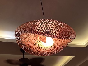
Just today, as I write this, I noticed an interestingly-shaped lampshade hanging from the ceiling (Figure 3.1). A lovely way to approach geometry is just to take time to stop and look at your surroundings, or perhaps display images for learners, and ask them to “Say what you see”. Attempting to capture the features of an object using increasingly precise mathematical language (e.g. plane, vertex, edge, face, parallel, perpendicular) can push learners to define terms more accurately. The teacher can also pose the mother of all questions, “What mathematical questions can you ask?”
Although we spend every day of our lives moving around in a 3D world, people often have difficulties with spatial awareness and struggle to imagine how an object would look from a different viewpoint. Simply walking around on earth for many years with our eyes open does not seem to be a reliable way to learn skills such as mental rotation. For example, parallel parking a car is well known to be a challenging task for many people.
I find that difficulties with spatial awareness seem to be just as common among professional mathematicians or mathematics teachers as anyone else, and this is something we can all work on getting better at. In schools, I often find that a young child will be dramatically better at this kind of thing than I am, so it is a nice opportunity to celebrate learners’ skills. Sometimes different learners excel in spatial learning than those who might do so with number and algebra. Many careers would seem to require a high level of spatial awareness, such as trades like building, carpentry, hairdressing and plumbing, as well as surgery, art and design, theatre and dance.
While 3D is our everyday reality, 2D (flat and curved surfaces) and 1D (lines and curves) are abstractions which do not perfectly exist in our world.3 A flat piece of paper has to have some small depth to it, otherwise it could not exist. Similarly, a line drawn, however thinly, on a surface must have some width, otherwise we wouldn’t be able to see it. And even the smallest dot representing a point must have some non-zero size, otherwise we would be unable to determine its location.
Despite this, we all seem to have little trouble imagining a Platonic world of perfectly straight lines that have no breadth, that continue indefinitely in both directions, and perfect circles that have no bumps or breaks. In the real world, we have to represent these abstractions by mathematical sketches that can never reproduce them exactly. However, the advantage of working with these imaginary abstractions, rather than reality, is that they are the simplest possible geometrical objects, and so reasoning about them is far more accessible than dealing with real-life objects. And often these abstractions can be excellent approximations to things that we do experience and care about in the actual world we live in (see Chapter 5).
3.3 Mathematical sketches
The impossibility of perfectly representing idealised mathematical objects, such as circles and lines, on real, physical paper raises the question of how we can work with these geometrical objects in practice and think about and discuss their properties with one another. One answer is to make mathematical sketches, and I think that it is worth being quite specific about what these are. I think learners are often confused about the status of the diagrams they see in books or on worksheets, and those that they produce themselves.
School teachers understandably often emphasise being ‘neat’ and ‘accurate’ in written and drawn mathematics. No teacher wants to have to struggle to decipher a confusing collection of words, symbols and scrawls in the learner’s notebook. And the teacher may pride themselves on the accuracy of their board-work in the classroom. However, while clarity of expression, orally, in writing, using symbols and making sketches, is a crucial aspect of mathematical communication, for me, ‘clear’ is quite different from ‘accurate’.
Consider this task:
Is this shape a square?

How would you go about answering this question? A learner might be inclined to say, “Yes”, and, if asked why, respond, “Because it looks like a square!”
They have seen a lot of squares in their life, and they believe they know one when they see one. But, of course, actually they have never seen a perfect square in their life, only approximations, and whether something is ‘approximately’ a square would depend on ‘how approximately’.
Another learner might say, “Yes, because it has four sides, all the same length and four right angles”. Is this a good answer?
Those are indeed necessary properties of a square, but do we know that this particular drawing has those properties? It certainly can’t have them with absolutely perfect accuracy.
A learner once brought a piece of paper to me on which they had drawn a shape like the one shown in Figure 3.2(a), but they held the paper in their hand so as to cover the top right portion, as in Figure 3.2(b). They asked me, “Is this a square?”

Suspecting something, I said, “I don’t know - I can’t see all of it!” But, even if I could have seen the entire drawing, and there was no ‘missing corner’, how could I have decided whether to say it was a square or not?
An interesting complication here is that a shape tends to look more like a square if you deliberately draw it slightly non-square. This is an optical illusion known as the vertical-horizontal illusion: an accurately-drawn square will look a little narrower than it is tall. This is possibly because a human’s horizontal visual field (the angular extent of what we can see in a horizontal plane by swivelling our eyes but not turning our heads) is typically wider than the vertical visual field. (The horizontal visual field is typically greater than \(180{^\circ}\), while the vertical one tends to be less than \(180{^\circ}\).) Optical illusions such as this can be a good way of convincing learners not to believe something “because it looks like it”.4
In trying to decide whether something like the shape in TASK 3.1 is a square or not, perhaps a learner would measure the lengths of the edges and the angles at the vertices using a ruler and angle measurer. But you can only ever make any measurement to a certain degree of accuracy. If our measurements suggest that the vertical sides might be \(1\) mm longer than the horizontal sides, is this enough for us to say “No”, or is that being too picky?
I have seen questions in teaching resources in which learners are asked to categorise drawn shapes as squares, rectangles, parallelograms, and so on, and really this is an impossible task. Maybe the drawn square in TASK 3.1 could be intended to represent a perfect square, but we can’t tell that by measurement - that depends on the intentions of whoever drew it. Really, I think it is an unmathematical question.
We cannot make this problem go away by ‘being more accurate’. In ‘the old days’, technical drawing was a marketable skill. As a teenager myself, I recall sitting in a roomful of drafting tables, learning how to draw accurate oblique parallel lines. Sometimes this sort of thing creeps into mathematics lessons under a heading of ‘scale drawing’ or ‘loci and constructions’, but it seems to me that such skills have become obsolete with the rise of modern technology. More importantly, this kind of accurate drawing work does not seem to me to have much to do with mathematics.
Scientists measure things, to specified degrees of accuracy. But mathematicians reason about geometrical properties, and rely on sketches that indicate relevant properties, rather than on accurate drawings. A mathematical sketch is accurate in the sense that it correctly indicates all the important features, but it does not aim to be accurate in their precise lengths and angles.
The kinds of drawings learners should be making in their mathematics lessons are always sketches. One way to emphasise this is to ask them to draw them freehand, rather than by using a ruler. This may not work for all learners, as some learners may have great difficulty in making an even approximately straight line without using a straight edge. And with very complicated geometrical sketches, a straight edge and pair of compasses are certainly very helpful for preventing everything from getting tangled up and confused. So, I would not ‘ban’ rulers. But, for illustrating the lines of symmetry of a square, say, a sketch like the one in Figure 3.3 is, in my opinion, ideal - and much quicker for learners to make than a more accurate drawing.

With a sketch like the one shown in Figure 3.3, we do not care if there are little wobbles, because we are trying to convey an idea, not make an accurate drawing. We can remind learners of this by asking them to ‘sketch’, rather than ‘draw’ their shapes, encouraging ‘clarity’ rather than ‘accuracy’.5 This allows them to work on a lot more mathematics in the same amount of time, and avoids spending time dealing with misplaced equipment. A lot of time is wasted in mathematics lessons making diagrams to a higher degree of accuracy than anyone needs in order to do the mathematics. Just because you can be more accurate doesn’t mean you should be (see Chapter 5). However, because the word ‘sketch’ is used differently in art lessons, some clarification will be needed.
Even when doing constructions with compasses and straight edge, the point is that these are ‘exact in principle’, and in my opinion the actual accuracy of any drawing the learner makes, perhaps with wobbly compasses and a worn-out bumpy ruler, is of little importance, provided the construction method is clear. Similarly, I am unconvinced that the skill of measuring and drawing angles using an angle measurer, say, is of much use for mathematics. Estimation based on paper-folding fractions of a straight line or right angle seem of much more value to me for understanding about angles.6
One very useful way to be able to show our meaning (e.g. to indicate an oblong versus a square) is to do our sketches on top of a squared grid, as in Figure 3.3. The general assumption when drawing on a grid is that we take the grid to consist of perfect squares, and when we draw a polygon, the edges are taken to be straight, and any vertices which appear to be at a grid point are taken to be exactly at the grid point. Using a grid, it is easy to show whether something is intended to represent a perfect square or an oblong (Figure 3.4).

And if we draw a figure like the one shown in Figure 3.5, we have a bit of work to do to justify whether it is a square or not. Remember, we cannot just rotate the page \(45{^\circ}\) and say, “Aha, now I see that it’s a square!” We have to reason that it is a square, not just say, “It must be a square, because it looks like one”, otherwise we are not doing mathematics. And to do this we need to have a definition of a square in terms of its essential properties, which we will come on to next.

The other nice thing about incorporating background grids is that we can bring in all the machinery of coordinate geometry. At an elementary level, this may just mean giving learners the opportunity to practise plotting coordinates for the vertices and describing lines of symmetry by using the equations of straight lines. But in more advanced work it often provides alternative methods of solution beyond classical geometry, by allowing solutions involving the algebra of the coordinate plane.
A nice task using a grid is the following:7
Look at the points \(A\), \(B\), \(C\), \(D\), \(E\), \(F\) and \(G\), shown below.
\(DEB\) is an isosceles right-angled triangle.
Make some similar statements using the other points.

Of course, not every polygon can be drawn with its vertices on a squared grid - an equilateral triangle is a simple and important example of a regular polygon which can’t. Isometric grids can be useful (Figure 3.6(a)), but on plain paper we can make little marks to indicate equality of length or angle (Figure 3.6(b)). These marks give us the advantage of being able to make diagrams that are deliberately drawn inaccurately.8 Often this can be helpful in avoiding giving away answers (which could be guessed at by eye or by rough measurement) and in helping learners not to trust in appearances.

Just because there is a grid, it doesn’t necessarily have to be marked off in specific units, such as centimetres. Centimetre-squared grids are very common and useful, as are \(5\) mm \(\times\) \(5\) mm grids, but we often prefer not to specify our units, and just treat the side length of each grid square as ‘\(1\) unit’. In that case, like on a number line, lengths are just dimensionless, pure numbers.
There is nothing wrong with saying that a line segment has a length of \(4\), or a square has an area of \(5\) or a prism has a volume of \(6\). This is not ‘forgetting the units’.9 Units are vital in applied contexts, in which the area is, say, the area of a football field or of a wall to be painted. In real-life applications, we certainly need to know if the area is \(20\) m2 or \(20\) square feet. But if we are doing a pure mathematics geometry problem, an area of \(20\) is just fine. Appending ‘squared units’ after the ‘\(20\)’ doesn’t achieve anything. Working in unspecified units makes our conclusions generalisable to any units we wish, from micrometres to light years.
3.4 Reasoning from properties
How would you describe the shape of the plate shown below?
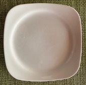
Everyone (including me) would call it a ‘square plate’. But it clearly has neither straight edges nor \(90{^\circ}\) angles. The issue here is not the one we discussed above, that no edge in the real world can ever be perfectly straight and no real angle can ever be precisely \(90{^\circ}\), and the plate is just as square as anyone could make it. On the contrary, this ‘square’ plate has very noticeably curved corners and edges, that the manufacturer never intended to be perfectly straight. And yet there is undoubtedly something ‘square’ about it, at least in comparison to the more usual circular variety.
Such a shape is sometimes called a squircle, and it is a good shape for a dinner plate, because a squircular plate has a larger area than a circular one with the same radius, but when you put it away in a rectangular cupboard it doesn’t take up any more room.
In a similar way, the UK Highway Code describes its warning signs as ‘triangular’ (e.g. Figure 3.7), which may be approximately true for the white region inside, but the outer red ‘triangle’ has noticeably rounded corners. It might even be called a ‘rounded triangle’.
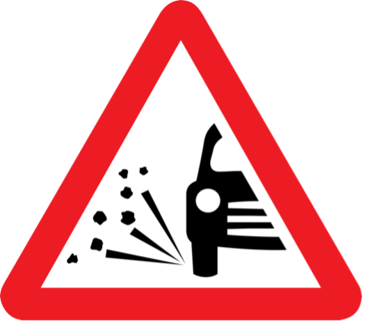
In everyday life it is fine to use language informally like this. But we have to do better in mathematics.
So, what exactly do we mean when we say that something is mathematically a square or a triangle? Returning to the tilted square I mentioned above (Figure 3.5), how do we reason that it is a square, given the usual assumptions about figures drawn on squared grids? The shape doesn’t fit neatly over a square arrangement of the given squares, because its edges pass diagonally through them.
This can be a good way to get learners to articulate their implicit knowledge about what a quadrilateral has to have to be a square, and this is quite a complicated definition, because it has to have both of two properties:
All edges are equal in length.
All vertices are equal in angle.
In fact, these two properties define regular polygons generally, and when applied to a \(4\)-sided polygon they define it as a square.
What matters in these kinds of discussions is the identification and articulation of relevant and essential properties. It is easy to spend far too much time focusing on naming shapes, because this is easy to test, and feels like a logical beginning. But if the teacher is not careful, so much time can be used up with this that we never get to examining the shapes themselves in much detail. Mike Askew has commented that the difficult words in mathematics are not really words like ‘parallelogram’ and ‘hypotenuse’, but words like ‘it’ and ‘has’ – that is the level at which complicated ideas are often found.10 In the van Hiele levels,11 which describe different stages in the learning of geometry, making general observations about shapes comes at the bottom and articulating formal deductions from precisely stated properties comes at the top.
I recently saw a professor of mathematics draw a sketch of the quadrilateral shown in Figure 3.8. “I think it has some special kind of name,” he said, “But I don’t remember what it’s called”.

I got the impression that not only did he not happen to recall the name, he didn’t much care about that. I thought this was interesting, because even quite young children are supposed to know that this shape is called a kite. Do they know something in mathematics that he doesn’t know?
It is often remarked on that people forget most of what they learn in school once they become adults. But we usually assume that is because they are no longer using those things from day to day. If the professor of mathematics had forgotten the date of the Battle of Waterloo, we might not be especially surprised. But since he spends all day every working day doing mathematics, shouldn’t we expect him to know this kind of thing?
Of course, perhaps it was just a momentary blank, which we all experience from time to time. But for me it reminded me that often the things that seem to get a lot of emphasis in school mathematics are different from the things that professionals who use mathematics give much weight to. Students might spend time learning ‘pentagon, hexagon, heptagon, …’, and their spellings, but a professional mathematician is more likely to say ‘\(5\)-gon, \(6\)-gon, \(7\)-gon, …’. This is effectively what these shapes are called in Greek. Is there any benefit to saying the names ‘in Greek’, rather than like this? It may be nice to know why the ‘Pentagon’ in Washington has that name, but there perhaps isn’t really much mathematics involved in spending too much precious classroom time on that kind of thing.
Something is going wrong if geometry lessons are mainly about naming things – what Gerry Leversha calls a sort of ‘natural history’ of geometry,12 like the old-fashioned biologists, who used to collect specimens and name them, but not really uncover much about their workings. They did observational rather than scientific work, that is sometimes referred to pejoratively as ‘stamp collecting’. Naming the polygons, and all the different kinds of quadrilaterals, and words associated with angles on parallel lines, and so on, can make geometry feel like a minefield of terminology.
Naming in geometry is useful only in so far as it enables some systematic classification of shapes. Children’s early experiences of shapes are often quite confused, with picture books using words like ‘diamond’ and ‘kite’ interchangeably, and treating a tilted square (Figure 3.5) as though it is not a square. When given a selection of different-looking quadrilaterals and asked to classify and name them, some learners created the names shown in the caption to Figure 3.9.

While names like these show thoughtfulness and creativity, inventing new, bespoke names ‘on the fly’ does not help us to appreciate where properties are shared and not shared among different shapes. The classic example of an unsystematic classification is the fictional ‘Celestial Emporium of Benevolent Knowledge’ animal taxonomy described by Jorge Luis Borges. This placed all animals into \(14\) categories:
those belonging to the Emperor, embalmed ones, trained ones, suckling pigs, mermaids (or sirens), fabled ones, stray dogs, those included in this classification, those that tremble as if they were mad, innumerable ones, those drawn with a very fine camel hair brush, et cetera, those that have just broken the vase, those that from afar look like flies.
It is a deliberate parody of people’s attempts to impose arbitrary and chaotic classifications on the world.
‘Dented triangle’ (Figure 3.9(a)) is an understandable, and actually quite memorable, name for an arrowhead. But mathematically it is unhelpful, because the name suggests the shape belongs to a subset of triangles, but since it has four sides it is not a triangle at all, but a quadrilateral.
The ‘half house’ (Figure 3.9(b)) is perhaps suggested by the proportions and orientation of the shape. Would the learner have invented that name if the shape had been presented stretched horizontally or rotated by \(90{^\circ}\)?
Sometimes, context is everything in the use of an informal name. Figure 3.10(a) is a rhombus, but if it is coloured red and placed near to a heart, a club and a spade, then we would call it a diamond instead (Figure 3.10(b)).13

Learners will often fail to recognise familiar shapes when they are in non-standard orientations, or they will recognise them, but think they have a different name. For example, a learner might call the tilted square in Figure 3.5 a ‘diamond’, rather than a square, just because of its unusual orientation. In mathematics resources, shapes are often drawn in mechanically stable-looking positions, with their longest side horizontal and at the bottom. A triangle drawn ‘point down’ may even be referred to as an ‘upside down’ triangle. It is good to subvert this, and instead offer learners a wider variety of different orientations.
We generally do not want mathematical names of shapes to depend on their colour or or orientation. We would say that an ‘upside down’ triangle (Figure 3.11(a)) is a perfectly acceptable triangle, and might claim that there is nothing ‘upside down’ about it, as a triangle can be in any orientation it likes. We tend to be slightly less consistent when it comes to 3D shapes, which are harder to imagine separate from the effects of gravity, and we do have ‘official’ terms like inverted pyramid (Figure 3.11(b)).14

One way to explore different polygons is to draw all the possible shapes of a certain kind that can be made on a \(9\)-pin geoboard (a \(3 \times 3\) square array of dots), in which all the vertices must be on dots. For example, there are \(16\) possible quadrilaterals, and learners can find and name them (Figure 3.12).

Another good way to become familiar with the properties of shapes is to play the card game Fourbidden.15
3.5 Inclusive definitions
One of the tricky - but very useful - things about mathematical definitions of shapes is the common use of inclusive definitions.16 For example, every square is a rhombus, but not every rhombus is a square.
I do not think it is so much the inclusive definitions that cause problems as learners’ pre-existing notions (concept images17) of the shapes.18 If the learner believes that the essential feature of a rhombus is its slanty look (Figure 3.13), then they will believe that it cannot have right-angled vertices, and therefore cannot be a square.

Sometimes learners will even think that the rhombus shown in Figure 3.14 is a ‘backwards rhombus’, because they are so used to rhombuses sloping to the right.

Similarly, a kite is any \(4\)-gon that has two pairs of adjacent equal sides. But would you go into a shop and buy a kite that looked like the one shown in Figure 3.15?

A nice way to address this issue is by presenting learners with repeated examples and non-examples of a shape, so that their preconceptions are systematically affirmed and challenged, until they are boxed into a happy corner with the correct concept definition.19
Inclusive definitions themselves are not actually at all unusual in learners’ worlds.
For example:
- Every cake is a dessert, but not every dessert is a cake. (It could be a rice pudding.)
- Every flower is a living thing, but not every living thing is a flower. (It could be a hippopotamus.)
- Every mathematics teacher is a teacher, but not every teacher is a mathematics teacher. (They could be an art teacher.)20
Examples like this are almost too obvious to need any comment, and if the teacher offers one or two, then learners will easily manufacture many more on demand. Then they can be invited to invent some which include given geometrical words, such as ‘kite’, ‘rhombus’, ‘parallelogram’ and ‘rectangle’.
Even very young children seem to have little difficulty with inclusive definitions themselves. For example, you might be playing ‘\(20\) Questions’ with a young child, to guess the child’s chosen object. If you ask, “Is it an animal?”, and they say “No”, then if sometime later you happen to ask, “Is it a bird?” they will instantly complain: “I already told you it wasn’t an animal!” Incidentally, ‘\(20\) Questions’ with a mathematical shape in mind can be an excellent activity for embedding these ideas.
The other important idea that tends to come up in association with inclusive definitions is the mathematician’s ‘if and only if’, which I also discussed in Chapter 2 in the context of divisibility. Learners’ first reaction to ‘if and only if’ is often to think that it just sounds like a pompous version of ‘if’, expanded for emphasis. Instead of a teacher saying, “I want each of you to do a drawing”, they could say “I want each and every one of you to do a drawing”. They have expanded out the word ‘each’ for dramatic effect, to stress that there are no exceptions, but the literal meaning of what they have said hasn’t changed.
‘If and only if’ is not like this. The ‘only if’ is just as meaningful as the ‘if’, and ‘if and only if’ is the combination of them both. I find that learners quite like knowing that it can be shortened to ‘iff’, with two f’s.
These correct statements below about a \(4\)-gon (quadrilateral) illustrate the difference between ‘if’ and ‘iff’:
Statement 1. A \(4\)-gon is a rhombus if it is a square.
Statement 2. A \(4\)-gon is a rhombus iff it has \(4\) equal sides.
The first statement tells us that the set of squares lies completely within the set of rhombuses.21 If you are in the squares, you are necessarily within the rhombuses, because ‘squares’ does not anywhere protrude outside of the ‘rhombuses’ region of a Venn diagram (Figure 3.16).

But there are rhombuses that are not squares - lots of them, in fact. These include the ‘classic’ rhombuses (such as in Figure 3.13) that do not have right-angled vertices. So, all squares are rhombuses, because all a rhombus needs to have is four equal sides, which all squares necessarily have. But not all rhombuses are squares - only the ones with right-angled vertices.
So, we cannot say:
- Statement 3. A \(4\)-gon is a square if it is a rhombus. (FALSE)
Statement 3 is not true, because lots of rhombuses are not squares.
But if we change it by adding ‘only’, then it is true:
- Statement 4. A \(4\)-gon is a square only if it is a rhombus.
Statement 4 is correct and is exactly equivalent to statement 1. The only \(4\)-gons that are squares are the rhombuses. It doesn’t say they all are. But a \(4\)-gon is a square only when it’s a rhombus, because any square has to also be a rhombus.
Learners may need to scratch their head and concentrate to get this. To be perfectly honest, I do too. I had to check back through this section carefully after I wrote it to make sure I hadn’t messed it up! It is easy for learners to think they have got this when they haven’t quite. The only thing that convinces me is to get them to explain repeatedly, in their own words, with different examples of their own making.
What is the Venn diagram that goes with statement 4? It is exactly the same one I drew in Figure 3.16. ‘A if B’ is exactly logically equivalent to ‘B only if A’. Because the squares all sit inside the rhombuses, a \(4\)-gon can be a square only if it is a rhombus. Something cannot be a member of the subset unless it is also a member the larger set that encompasses the subset.
Going back to statement 2 above, ‘if and only if’ means ‘if’ both ways!
A \(4\)-gon is a rhombus if it has \(4\) equal sides, and a \(4\)-gon has \(4\) equal sides if it is a rhombus. ‘If and only if’ is just a shortened way of making both of these statements, without having to write out the words twice.
We could imagine the ‘if’ and the ‘only if’ as separate Venn diagrams (Figure 3.17). The only way both of these can be true is if ‘a rhombus’ and ‘\(4\) equal sides’ are equivalent properties - you can’t have one without the other. For this reason, definitions are ‘if and only if’ statements. They don’t merely say that something is an example of some larger class; they tightly prescribe the limits of it by saying what it is exactly equivalent to. So, statement 2 is a definition of a rhombus: a \(4\)-gon that has \(4\) equal sides.

In ordinary life, ‘if’ is sometimes taken to mean ‘if and only if’, but children love being pedantic, so I don’t think this is a problem as often as is usually claimed. For example, someone might say, “If you come to my birthday party, you can have some birthday cake.” The invitee might assume from this that if they do not attend the party they will not receive any birthday cake. But that isn’t actually what the person said, and it is possible that if they don’t attend the party then they could perhaps call in the next day and pick up a piece of cake.
With “If you sign the contract, then we will do business”, the ‘if and only if’ implication feels a bit stronger. But a bare ‘if’ still leaves the possibility of doing business without the contract, or with some alternative contract in place instead. “If and only if you sign the contract, we will do business” is an ultimatum that there will be no doing business without this contract being signed. But, alongside this, it is also a promise that business will be done if this contract is signed. ‘If and only if’ is always making two parallel statements like this, just as the contract delivers rights and obligations to both parties.
The purpose of inclusive definitions is to reduce the number of theorems we need to have.
For example, the two diagonals of a rectangle bisect each other, and so do the diagonals of a rhombus (Figure 3.18).

Actually, the diagonals of a parallelogram also bisect each other, and so do the diagonals of a square. How can we remember all this?
Well, if a square is a rhombus, and a rhombus is a parallelogram, and a square is a rectangle, and a rectangle is also a parallelogram, then if we use inclusive definitions we just need one theorem:
- Theorem 3.1. The diagonals of a parallelogram bisect each other.
And then that one theorem includes all the other theorems as special cases, which is a great saving.
Here is another theorem:
- Theorem 3.2. The diagonals of a kite intersect at right angles.
What follows from this?
Because a rhombus is a kite (because it has two pairs of adjacent equal sides), its diagonals must also intersect at right angles. And this must apply to a square too, because a square is a rhombus. And a rhombus (and also a square) is also a parallelogram, and so Theorem 1 must also apply. So, the diagonals of a rhombus bisect each other, and do so at right angles. We get all these conclusions with minimal effort, because we use inclusive definitions. We would always rather have one more general theorem than lots of separate little theorems that apply in specific cases.
A very nice way to represent the different quadrilaterals is to use John Ling’s clever idea of making a Venn diagram in which each region takes the form of the shape that it represents (Figure 3.19).

People often say that the value of inclusive definitions is that any fact that is true for the larger category is true for every sub-category too. That is usually the case, as in these examples with intersecting and bisecting diagonals. Objects in the sub-category can have additional properties - for example, a square has four equal sides, but a parallelogram (which contains all the squares) doesn’t necessarily. But there shouldn’t be any property of a parallelogram which a square doesn’t also share.
However, in fact, there are such properties, particularly when it comes to symmetry.
For example, a general (non-rectangular, non-rhombus) parallelogram has no lines of symmetry. Learners often think that the dashed line shown in Figure 3.20(a) is a line of symmetry, but if you reflect the left-hand portion of that figure in that line, you do not complete the parallelogram (Figure 3.20(b)). (I have often found that cutting out the shape from paper and folding it is often necessary to convince learners of this.)

A rhombus always has two lines of symmetry, through its vertices (Figure 3.21(a)), and a rhombus that is also a square has two more lines of symmetry, through the midpoints of the opposite sides (Figure 3.21(b)). You could say here that the subsets of shapes (e.g. the squares) just have additional properties (extra lines of symmetry). But if we treat ‘the number of lines of symmetry’ as a property, then ‘having zero lines of symmetry’ (e.g. a general parallelogram) is a property that the squares don’t have.
This is perhaps even more clear cut when it comes to order of rotational symmetry. A non-square parallelogram has order \(2\), but a square (which is necessarily also a parallelogram) has order \(4\). Mathematics teaching resources will sometimes ask questions like, “What is the order of rotational symmetry of a parallelogram?” without realising that the writer has in mind a non-square parallelogram. Otherwise, the answer would have to be “\(2\) or \(4\), depending on what kind of parallelogram it is”, which is never what you see when you look at the answers in the back of the book!

There is also sometimes disagreement over which inclusive definitions should be used. Is a parallelogram also a trapezium? Is an equilateral triangle also an isosceles triangle? I would say yes to both, but others think differently.
It is also worth noting that there are shapes that are defined outside this inclusive, hierarchical system; in particular, an oblong is simply a non-square rectangle, so we can say that an oblong has two lines of symmetry, even though a rectangle may have two or four, depending on whether it is a square rectangle or not.23
3.6 Angles
3.6.1 The notion of angle
Angle is quite a tricky idea.24 All of the angles drawn in Figure 3.22 are equal, but they may not look it to learners.

Cutting them out of paper and overlaying them on top of each other could help to demonstrate this. In particular, learners need to learn to disregard the length of the straight ‘arms’, either side of the angle itself.
We saw in Chapter 1 that when a shape is scaled up to make a similar shape, its angles do not change. To help learners get a sense of angle by using angle measurers, empty (i.e. unscaled) protractors can be very helpful.25
Visualising angle dynamically, as a measure of turn, can be achieved by having learners stand up and all face some common reference direction, such as the front of the room. Learners can then be asked to turn clockwise or anticlockwise physically by different amounts - perhaps with their eyes closed, so as not to be influenced by their peers’ movements. The amount of turn could be stated first in terms of fractions of a full turn,26 and, later, once we attach the arbitrary number \(360\) degrees (\(360{^\circ}\)) to one complete turn, as various numbers of degrees (Figure 3.23).27 Referencing learners’ experiences on playground roundabouts may be helpful.

Through careful choice of the angles requested, learners will notice, for example, that a clockwise turn through \(120{^\circ}\) reaches the same position as an anticlockwise turn through \(240{^\circ}\), and they might generalise this to angles \(n\) and \(360{^\circ} - n\).
They might also notice, for example, that an anticlockwise turn through \(1000{^\circ}\) corresponds to a clockwise turn through \(80{^\circ}\). In general, a clockwise turn of \(c\) is equivalent to an anticlockwise turn of \(a\) if and only if
\[c\ \text{mod}\ 360{^\circ} = - a\ \text{mod}\ 360{^\circ}, \qquad \text{ or } \qquad (a + c)\ \text{mod}\ 360{^\circ} = 0,\]
where ‘\(\text{mod}\ 360{^\circ}\)’ refers to taking the remainder after dividing by \(360{^\circ}\) (e.g. \(370{^\circ}\ \text{mod}\ 360{^\circ} = 10{^\circ}\)).
The modular arithmetic (Chapter 4) behaviour of angles is similar to that with time in hours, which is ‘mod \(12\)’ (for \(12\)-hour clock) or ‘mod \(24\)’ (for \(24\)-hour clock). This is why an analogue clockface is so suitable for representing time.
For example, \(9\) hours after \(8{:}00\) pm (\(20{:}00\) hours) is \(5{:}00\) am.
We can write
\[20{:}00 + 9 \text{ hours }= 05{:}00,\]
and this works because \(20 + 9 = 29 = 5\ \text{mod}\ 24\).
Similarly, minutes and hours are \(\text{mod}\ 60\).
In a similar way, days of the week are ‘\(\text{mod}\ 7\)’, so, for example, \(25\) days after a Tuesday will be the same day of the week as \(25\ \text{mod}\ 7 = 4\) days after a Tuesday, so it will be a Saturday. Modular arithmetic, even if not stated in those terms, has many applications in daily life.
Learners can try to estimate the sizes of some everyday angles, such as the horizontal angle of their field of vision (the angle they can look through without turning their head) and the angle they turn a particular door handle to open it. Most learners will overestimate the angle of everyday slopes: walking up or down a slope of even \(30{^\circ}\) is difficult. They might enjoy improving their angle estimation skills with a game.28
A nice task involving angles, that only requires knowing that a full turn is \(360{^\circ}\), is to consider the angles made between the hands on an analogue clock at different times:29
At what times are the hour and minute hands on a clock at right angles to each other?
Find a way to calculate the angle between the hour hand and the minute hand at any given time.

Learners will often suggest that the clock hands make a right angle at times such as \(09\text{:}30\), but this is not exactly correct, because the hour hand will not be pointing exactly at the \(9\), but half way between the \(9\) and the \(10\).30 There are many interesting related angle problems involving clocks.31
Once we have decided that ‘all the way round’ is \(360{^\circ}\), then a straight angle, being half of this, must be \(180{^\circ}\), and so any angles that fit together along a straight line will have a sum of \(180{^\circ}\): we call them supplementary angles.
It is worth mentioning that the converse is also true: if two angles sum to \(180{^\circ}\), then when placed next to each other they will make a straight line.
3.6.2 Vertically opposite angles
There is a nice bit of reasoning to deduce that vertically opposite angles (i.e. opposite angles at a ‘vertex’) are equal (Figure 3.24).
The top black angle in Figure 3.24(a) and the left-hand white angle together make a straight angle, so are supplementary. And, similarly, the top black angle and the right-hand white angle are also supplementary, since they also fit together on a straight line. Since each of the white angles is the difference between \(180{^\circ}\) and the top black angle, the two white angles must be equal to each other.


An identical argument shows that the two black angles must be equal to each other.
I think doing this without using any algebra highlights the simplicity of the reasoning. Like opening and closing a pair of scissors, as the two black angles decrease, the two white angles must increase, degree for degree, and vice versa.
3.6.3 Corresponding and alternate angles
I do not think it is worth trying to ‘prove’ why alternate or corresponding angles are equal, because it inevitably has to depend on something that is less obvious than what we are trying to prove. An informal argument about translating (for corresponding angles) or rotating (for alternate angles) one angle onto the other, should be enough to convince learners that they can use these results and their converses (i.e. that if the relevant angles are equal, then the lines must be parallel) (Figure 3.25 and Figure 3.26).


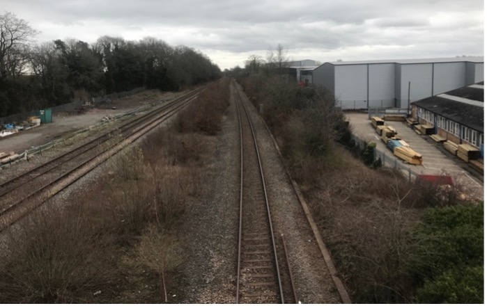
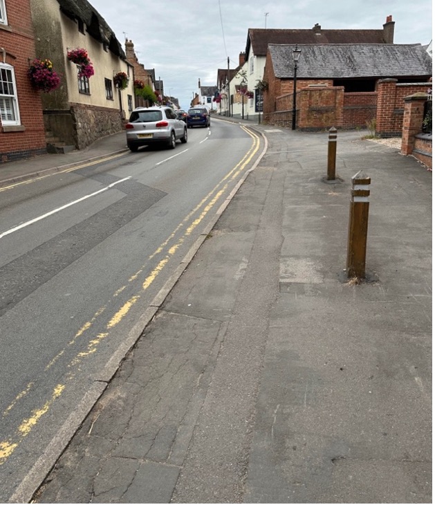
An informal understanding of what ‘parallel’ means is sufficient for school geometry. Parallel lines are straight lines that go ‘in the same direction’ and are always the same distance apart. Train tracks and double yellow lines are not necessarily parallel lines, because they often go in curves (Figure 3.27). They can be called parallel curves.
3.7 Triangles
Having explored this general thinking around different 2D shapes and learners’ understanding of angles, there are really only two categories of 2D shape that are particularly important in school mathematics: triangles and circles. Despite the multitude of different names for them, quadrilaterals do not turn out to be particularly important. If learners are familiar with the key properties of both triangles and circles, they will have a lot of geometric power, and a solid basis for dealing with anything else they might meet in geometry.
In school mathematics, we are rarely precise about what we mean when we refer to a shape such as a ‘triangle’. Literally, ‘triangle’ means ‘three angles’, referring to the three vertices. Sometimes, by ‘triangle’ we mean the three connected edges (sides), and sometimes (such as when we say ‘the area of a triangle’) we mean the interior space, surrounded by the three edges, and perhaps including the edges as well. It is usually obvious by the context what is meant. Unlike with the names ‘circle’ and ‘disc’, with polygons we do not have different terminology for the boundary and the interior.
Learners can practise using language such as scalene, isosceles, equilateral, acute-angled, right-angled and obtuse-angled to describe triangles by trying to find examples of these in interesting-looking shapes.
For example, Figure 3.28(a) shows a regular pentagon with all its diagonals drawn (or we can think of it as a pentagram inscribed within a regular pentagon). If learners count systematically, they will find \(35\) triangles in total, of various kinds.

For the regular hexagon in Figure 3.28(b), there are \(110\) triangles, which is too many to count them all.32 But in the regular hexagon they can find examples of right-angled triangles, which Figure 3.28(a) did not include.
Another task that achieves this is the following:
Find all the different triangles that can be made on a \(9\)-pin geoboard (a \(3 \times 3\) square array of dots), in which all the vertices must be on dots.
There are \(8\) possible triangles, and learners can find and name them (Figure 3.29).

3.7.1 The interior angle sum of a triangle
The most basic theorem about a triangle is probably that its interior angle sum is \(180{^\circ}\). This follows from the useful theorem that any exterior angle of a triangle is equal to the sum of the two opposite interior angles (Figure 3.30).

This is our first example of a theorem that can be proved by the tactic of the addition of a single auxiliary line, shown dashed in Figure 3.30.33 By judiciously choosing this auxiliary line to be parallel to one side of the triangle, we create alternate angles, which are equal (light grey), and also corresponding angles (dark grey), which are also equal to each other. So, we can literally see (without any words) the two opposite angles summing to the given exterior angle. We will see many other examples of auxiliary lines coming to the rescue like this.34
Since each exterior angle (like all exterior angles) is adjacent to the interior angle at the same vertex, they are supplementary (their sum is \(180{^\circ}\)), and so it follows that the sum of the three angles in the triangle is also \(180{^\circ}\). We can see in Figure 3.30 the white, the light grey and the dark grey angles all fitting together on a straight line.
Another way to show this is to fold one vertex along a line joining the midpoints of two of the sides, and then fold the other vertices to meet the first one (Figure 3.31).

Dynamic geometry is very convenient for convincing learners that we have proved this result generally, and not just for this specific triangle. However we wiggle the top vertex, as one of the angles increases, the others will change accordingly. If we keep the white angle constant, say, and increase the dark grey angle by \(1{^\circ}\), the light grey angle must decrease by \(1{^\circ}\) to keep the sum of all three angles constant. The result will remain true for any triangle we can imagine, and this is the essence of a general deductive proof. It is easy to assume that learners appreciate this when they don’t.
3.7.2 The exterior angle sum of a triangle
Learners are often confused about the fact that the exterior angle at a vertex is not the entirety of the angle at that point, less the interior angle (Figure 3.32). We might call such an angle the ‘external’ angle at the vertex, but it is not the exterior angle.

This ‘external’ angle is explementary (or conjugate) to the interior angle, meaning that they sum to \(360{^\circ}\), whereas the true exterior angle is supplementary to the interior angle at that vertex (they sum to \(180{^\circ}\)).
The sum of these ‘external’ angles will be \(3 \times 360{^\circ} - 180{^\circ}\), which is \(900{^\circ}\), but the sum of the actual exterior angles will be less by \(180{^\circ}\) for each vertex, which is \(900{^\circ} - 3 \times 180{^\circ} = 360{^\circ}\).
Each anticlockwise exterior angle is equal to the clockwise exterior angle at the same vertex, because they are vertically opposite each other (Figure 3.33).

Because each exterior angle is the sum of the two opposite interior ones, if we sum all three exterior angles, then we sum all three interior angles twice. This means that the sum of the exterior angles of a triangle must be \(2 \times 180{^\circ} = 360{^\circ}\).
We can see the exterior angle sum more easily just by zooming out on a general triangle and looking at the exterior angles (Figure 3.34).

3.7.3 Interior and exterior angles of polygons
Once we know about the interior and exterior angles of a triangle, we have effectively solved the problem for all polygons, because all polygons can be considered as being composed of triangles.
Any convex \(n\)-gon from a \(4\)-gon upwards can always be dissected into \(n - 2\) triangles by joining any vertex to all the \(n - 3\) vertices that that vertex is not yet joined to. Each vertex is already joined to its \(2\) neighbouring vertices, leaving all of the \(n\) vertices besides itself and its \(2\) neighbours, which is \(n - 3\) vertices.
Drawing \(n - 3\) new diagonal lines creates \(1\) more triangle than this, so \(n - 2\) triangles. Here, again, we are adding auxiliary lines to our shape (shown dashed in Figure 3.35) to enable a solution. The total interior angle sum of these \(n - 2\) triangles will be \(180(n - 2){^\circ}\).

Splitting the polygon into triangles is a convenience, rather than a necessity.
If we already know that a quadrilateral (since it is composed of two triangles) has an interior angle sum of \(2 \times 180{^\circ} = 360{^\circ}\), then we can split polygons into combinations of triangles, quadrilaterals, and any other polygons we already know the interior angle sum of. We will always obtain the same total interior angle whichever way we do it.
For example, a \(5\)-gon can be three triangles (\(3 \times 180{^\circ}\)) (Figure 3.35) or one triangle and one quadrilateral (\(180{^\circ} + 360{^\circ})\) (Figure 3.36), but either way it will come to \(540{^\circ}\).

It can even be \(5\) triangles, provided we remove the excess \(360{^\circ}\) angle created in the middle, because \(5 \times 180{^\circ} - 360{^\circ} = 540{^\circ}\) (Figure 3.37).

The exterior angles are easier than the interior ones, at least for a convex \(n\)-gon, because we can just imagine walking around the perimeter, which involves turning through the exterior angle at each vertex as we go (Figure 3.38).35 (For this reason, exterior angles are sometimes referred to as turn angles.)

Since this takes us through \(360{^\circ}\) and back to facing in the same direction we began in, this means that the sum of all of the exterior angles of any convex \(n\)-gon must be \(360{^\circ}\) (Figure 3.39).36

In Figure 3.40, we imagine sliding all these exterior angles to a single point. Alternatively, we can imagine zooming out, until the polygon itself is too small to see, and all we see are the angles, making a full turn.

It is perhaps surprising that the total angle doesn’t depend on the number of vertices. The more vertices there are, the less we can afford to turn at each one, if we are to get through \(360{^\circ}\) by the time we get back to the start.
For a concave polygon, we would have to count some of the exterior angles as negative, because we turn in the opposite sense (clockwise/anticlockwise), but if we do so then the total exterior angle still comes to \(360{^\circ}\).
Logo37 is a fantastic piece of free software for exploring interior and exterior angles of polygons, by using commands such as ‘forward’ and ‘right’ to control the movements of a ‘turtle’. If you ask learners to draw a square, they will have no difficulty constructing code such as that shown in Figure 3.41(a). However, when they try something similar to make an equilateral triangle, they will often produce something like the code shown in Figure 3.41(b).

However, although the code for the square will work, the code for the equilateral triangle will not produce the desired equilateral triangle, but instead will make half of a regular hexagon (Figure 3.42), because the angles that the turtle turns through are the exterior angles, rather than the interior ones.
The surprise of this can be memorable, and learners will need to change both \(60{^\circ}\) angles into \(120{^\circ}\) angles to correct their code. The fact that in the case of rectangles, exterior angles are equal to interior angles, can contribute to this confusion.

3.7.4 Congruence
The really useful feature of triangles in geometry is the same thing that makes them useful in construction, and that is their rigidity. In other words, if you know the lengths of the three sides of a triangle, then that fixes the three angles. Once you have made your triangle using your three lengths, there is no wobbling it around into differently shaped triangles.
This contrasts with a quadrilateral, which is not rigid, unless you put in a diagonal strut, effectively making it into two (rigid) triangles. The two quadrilaterals in Figure 3.43 have the same four side lengths. But the dashed diagonal in the first one will not span the corresponding vertices in the second one.

Formally, we say that SSS (side-side-side) is a condition for congruency, meaning that two triangles are exactly the same as each other, except possibly for a reflection.
Using compasses to construct triangles given the three side lengths will lead learners to realise that, if the triangle exists, there is a unique position for the ‘final’ vertex (Figure 3.44(a)). However, if two of the sides sum to less than the third, then the two arcs will not intersect, and there is no such triangle (Figure 3.44(b)).

Learners are often shocked to discover that you can’t necessarily make a triangle out of any three arbitrary lengths. But if the teacher suggests three lengths, such as \(100\) cm, \(2\) cm and \(3\) cm, they will quickly see the problem. The fact that three lengths \(a \leq b \leq c\) will make a triangle if and only if \(a + b > c\) is called the triangle inequality.
There are two other congruency conditions, which are equivalent to this one.
One is SAS (side-angle-side), where the angle is the angle in between the two sides - that is why the letters are written in that order. Once you fix SAS, the remaining side is forced to go in the gap between the open ends of the other two sides, shown dashed in Figure 3.45.

Finally, ASA begins with a fixed side length, and then lines come off each end at fixed angles \(A_{1}\) and \(A_{2}\), which are forced to meet at a unique point, which must be the location of the third vertex (Figure 3.46).

Any combination of a side and two angles is equivalent to ASA, because if we have any two angles we can always find the third one, using the fact that the interior angle sum of a triangle is \(180{^\circ}\). This means that AAS is just as valid a congruency condition as ASA.
The one to watch out for, which is not a congruency, is SSA. Unlike two angles and a side, which does fix a triangle uniquely, two sides and an angle is sometimes ambiguous. In some cases, there are two possible triangles that fit the same side-side-angle condition.
For example, in Figure 3.47(a) there are two possible positions where the side \(S_{2}\) can meet the horizontal dashed line, leading to two different possible triangles, shown on the right.

However, if \(S_{2}\) happens to be precisely the right length (namely, equal to \(S_{1}\sin A\)), then the circle in Figure 3.47(a) will be a tangent to the horizontal dashed line, and we will get just one, right-angled triangle (Figure 3.48(a)).

So, if SSA becomes right-angle-side-hypotenuse (RSH), then we do have a condition for congruency. (Equivalently, since this is a right-angled triangle, a hypotenuse and a leg determine the other leg, by Pythagoras’ Theorem, and so RSH can also be thought of as just SSS.)
Finally, if \(S_{2} < S_{1}\sin A\), then the circle won’t be able to meet the dashed line, and we don’t get a triangle at all (Figure 3.48(b)).
Throughout all this discussion, the interplay between circles and triangles is central. As we will see shortly, circles give us all the places that are some fixed, straight-line distance from a fixed point. Compass-and-straight-edge constructions are the ideal way to see this.38
3.7.5 Trigonometry
3.7.5.1 Sine, cosine and tangent
We saw in Chapter 1 that trigonometry can be viewed as being about multipliers within triangles, but we can also link this to circles, bridging these two crucial categories of shape.39
We can define \(\cos\theta\) and \(\sin\theta\) as the lengths of the sides of the right-angled triangle inside a unit circle, as shown in Figure 3.49.40 As \(\theta\) varies, these lengths vary, and if we expand or contract the circle, so that it has a radius other than \(1\), everything scales by this radius multiplier, just as we saw in Chapter 1.

We considered similar triangles in Chapter 1, viewing the between-triangle ratios of corresponding sides as a scale factor (i.e. multiplier). This is analogous to seeing the radius of the circle as the multiplier \(r\) when switching between \(\sin\theta\) and \(r\sin\theta\) or \(\cos\theta\) and \(r\cos\theta\).
We also thought of the within-triangle side ratios as multipliers, and in right-angled triangles these had special names – sine, cosine and tangent – and values we could find on a calculator, if we knew one of the acute angles.
If we understand thinking multiplicatively, when given two similar triangles, we can always find any missing side in one triangle if we know the corresponding side in the other triangle and the scale factor. Alternatively, we can find the length of any side in a right-angled triangle if we know one of the acute angles and one of the other sides.41
3.7.5.2 The sine rule
The sine rule generalises trigonometry beyond right-angled triangles, based on the observation that the largest angle is always opposite the largest side.42
If \(A \leq B \leq C\) then \(a \leq b \leq c\), and vice versa (Figure 3.50).

More precisely,
\[\dfrac{\text{side length}}{\text{sine of the angle}}\]
is a constant for any particular triangle.43
This is more usually written as
\[\dfrac{a}{\sin A} = \dfrac{b}{\sin B} = \dfrac{c}{\sin C} ,\]
which reduces to the standard definition of \(\sin A\) if either \(B\) or \(C\) becomes \(90{^\circ}\).
Learners often find it peculiar that this formula contains two equals signs. They might even have been told that it is wrong to write two equals signs on the same line as each other (see Chapter 2).
Really, this formula is just saying that \[s \propto \sin\theta\] for each side \(s\) and opposite angle \(\theta\), with the same constant of proportionality for the same triangle. There are two equals signs, just because the triangle has three sides.
With a formula like this, learners should worry about whether we could ever obtain a sine value greater than \(1\), since this should be impossible.
Since
\[\sin B = \dfrac{b\sin A}{a} ,\]
what would happen if, say, \(\sin A = 0.9\), \(b = 5\) and \(a = 3\)?
Then,
\[\sin B = \dfrac{b\sin A}{a} = \dfrac{5 \times 0.9}{3} = 1.5 .\]
Because \(- 1 \leq \sin B \leq 1\), a value of \(1.5\) is impossible, and the inverse sine function on the calculator will give an error if we try to make it find the inverse sine of \(1.5\). Is there some reason why this could never happen when using the sine rule?
Let’s see what the triangle would have to look like to generate this impossible calculation.
If \(\sin A = 0.9\), then according to the calculator, angle \(A\) must be about \(64.2{^\circ}\) (correct to \(1\) decimal place). Figure 3.51 shows a sketch. Does anything seem obviously wrong in this sketch?

We are trying to draw SSA, consisting of a \(64.2{^\circ}\) angle, followed by a \(5\) cm side, followed by a \(3\) cm side.
We saw before, when we thought about congruency, that SSA sometimes gives two possible triangles, sometimes one and sometimes none. Here, because \(5\sin{64.2} = 4.5 > 3\), the \(5\) cm side is too long for the \(3\) cm to make it back to the horizontal, whatever the size of angle \(C\). In other words, there is no such triangle as this one, as is shown in Figure 3.52.

Looking back at Figure 3.51 now, we can maybe see that we should have been suspicious. The angle of \(64.2{^\circ}\) is opposite the side of length \(3\), and so the angle opposite the side of length \(5\) must be even larger than this. That means we have less than \(180{^\circ}-2\times64.2{^\circ}\), which is only about \(52{^\circ}\), left for angle \(C\), which may seem implausibly small.
This is quite a subtle point, and occasionally textbooks and examination papers have unintentionally included calculations on impossible triangles like this one, that do not actually exist, without anyone noticing before they were printed! Some teachers might say that a discussion like this is ‘just confusing the learners’. On the other hand, seeing why the formulae that we use work, and how they are not going to go wrong, no matter what we do to them, can be very helpful. It is reassuring to see that impossible things are not going to suddenly happen!
3.7.5.3 Pythagoras’ Theorem
Pythagoras’ Theorem is one of my favourite topics within the whole of the school mathematics curriculum. It is a genuinely surprising and intriguing result that we should not have expected to be true or to be so simply expressible. There is no comparison between the importance of Pythagoras’ Theorem and, say, something like the formula for the volume of a cone or a sphere. Learners may think of all of these as ‘just another formula to substitute into’, and we need to help them to see more deeply than this.
A really nice way to introduce Pythagoras’ Theorem is Tom Francome’s idea of taking cut-out squares of different integer areas, and using three of them at a time to create a triangle (e.g. Figure 3.54).44

Sometimes it is impossible to make a triangle from three squares (e.g. Figure 3.54). This happens when the sum of the two shorter sides is less than the longest side, meaning there is no way for them to reach to connect up and make a triangle (the triangle inequality that we saw in Section 3.7.4).

However, when it is possible to make a triangle, learners will notice that sometimes these triangles appear to be right-angled, which is easy to spot without needing to use a protractor, because of the right-angles inside the squares (e.g. Figure 3.55).

Other times, the triangles appear to be acute-angled or obtuse-angled. A little bit of categorising allows us to notice that the right-angled triangles seem to appear when the areas of the two smaller squares add up to the area of the larger square.
When the areas of the two smaller squares sum to less than the area of the largest square, the triangle will be obtuse-angled, like the triangle made from squares with areas \(5\), \(13\) and \(26\) shown in Figure 3.54.
When the areas of the two smaller squares sum to more than the area of the largest square, the triangle will be acute-angled, like the triangle made from squares with areas \(5\), \(8\) and \(9\) shown in Figure 3.56.

It is easy for learners to distinguish acute-angled, obtuse-angled and right-angled without using angle measurers, and just by looking (or by poking the right-angled corner of a piece of paper into the triangle to compare, if they are not sure).
From this, we could conjecture that
- \(a^{2} + b^{2} > c^{2}\) for acute-angled triangles,
- \(a^{2} + b^{2} = c^{2}\) for right-angled triangles,
- \(a^{2} + b^{2} < c^{2}\) for obtuse-angled triangles.
Of course, we cannot be sure that this is precisely true just by looking at our shapes, and, for convenience, we have only tried a few examples, and they have all involved squares with integer area.
So, we need to prove that the relation \(a^{2} + b^{2} = c^{2}\) applies precisely to any right-angled triangle with legs \(a\) and \(b\) and hypotenuse \(c\).
The easiest proof is to make a square shape from four copies of the triangle and a tilted square for \(c^{2}\), as in Figure 3.57(a).

The area of each triangle is \(\dfrac{1}{2}ab\), but there is no need even to work this out, because all we need to do is slide the four triangles within the large square, leaving the white space where the \(c^{2}\) was, now equal to \(a^{2} + b^{2}\), as in Figure 3.57(b).
To be precise, learners should satisfy themselves that the three white quadrilaterals are all squares. Notice that we tacitly assume that translations don’t change area.
Using Pythagoras’ Theorem to find the lengths of legs and hypotenuses of triangles involves switching between the ‘area world’ of the formula \(a^{2} + b^{2} = c^{2}\) (a sum of two areas is equal to another area) and the ‘length world’ of \(a\), \(b\) and \(c\).
It would be possible to present Pythagoras’ Theorem instead, purely in the length world, as two formulae:
- \(c = \sqrt{a^{2} + b^{2}}\) for finding a hypotenuse, and
- \(a = \sqrt{c^{2} - b^{2}}\) (or, equivalently, \(b = \sqrt{c^{2} - a^{2}}\)) for finding a leg.
However, to me this feels much less elegant, and leads to more separate things for learners to remember. Rearranging formulae is a valuable goal in itself (Chapter 2), not only for mathematics but for science. So, I prefer to stick with the overall result \(a^{2} + b^{2} = c^{2}\), and support learners in dealing with this flexibly, depending on what they need to calculate.
The converse of Pythagoras’ Theorem is also true, and is sometimes assumed without being proved or even discussed.45
3.7.5.4 The cosine rule
We dealt earlier with the sine rule, and now we can think of the cosine rule as a mere ‘correction’ to Pythagoras’ Theorem for non-right-angled triangles. The word ‘correction’ here is not meant to imply any fault or inaccuracy with Pythagoras’ Theorem – no offence to Pythagoras! Perhaps ‘generalisation’ might be a better term than ‘correction’.
If \(a\), \(b\) and \(c\) are the side lengths of any triangle, with \(A\), \(B\) and \(C\) the angles in degrees opposite these (angle \(C\) not necessarily \(90{^\circ}\)), as we had back in Figure 3.50, then in general
\[a^{2} + b^{2} = c^{2} + 2ab\cos C .\]
If \(C = 90{^\circ}\), then \(\cos C = 0\), and the new term disappears, leaving us with Pythagoras’ Theorem, \(a^{2} + b^{2} = c^{2}\).
If \(C < 90{^\circ}\) (an acute-angled triangle), then \(\cos C > 0\), making the \(2ab\cos C\) term positive (since \(a\) and \(b\) are lengths, which have to be positive). This reduces the side length \(c\), relative to \(a\) and \(b\), as it must, since angle \(C\) is smaller.
If \(C > 90{^\circ}\) (an obtuse-angled triangle), then \(\cos C < 0\), making the \(2ab\cos C\) term negative. This increases the side length \(c\), relative to \(a\) and \(b\), which is as we expect, since angle \(C\) is now greater than \(90{^\circ}\).
In addition to proving the cosine rule, spending a few minutes thinking about how it relates to learners’ observations of acute-angled and obtuse-angled triangles, and Pythagoras’ Theorem, feels important.
The cosine rule is useful when you are given SAS and want to find the remaining side or one of the remaining angles. It is also useful if you have SSS and want to find one of the angles. In all other cases, the sine rule tends to be more convenient.
3.7.6 Area and Perimeter
Area and perimeter are often confused, even though they are very distinct quantities with different dimensions (and units). Comparing and contrasting their features is important.46
3.7.6.1 Area of polygons
Because of their rigidity, triangles are also very useful for calculating areas of more complicated shapes. We can always split up a polygon into non-overlapping triangles (a tessellation or tiling), and the total area of the polygon will be the sum of the areas of the triangles.
Learners are often asked to calculate area and perimeter of rectilinear shapes (shapes whose angles are all right-angles), such as U or L shapes, where decomposing into rectangles may be more convenient. It is also easier with some polygons to enclose them in a rectangle and find the desired area by subtracting off the triangles or rectangles created around the edge (Figure 3.58).

Every triangle can be obtained from a parallelogram by making one straight symmetrical cut along the diagonal, and so every triangle area is half that of the corresponding parallelogram, which is just a shear of a rectangle (Figure 3.59).47

Shearing is a very useful transformation, that is area-preserving - something that is easily suggested by pushing over a pile of books or sheets of paper (Figure 3.60).48

The multiplier of \(\dfrac{1}{2}\) in ‘half the base times the height’ for the area of a triangle sometimes confuses learners. “Is it half of the base, timesed by the height, or half of the whole thing?” The answer to this is ‘yes’ – it is both, and this is a nice example of the associativity of multiplication:
\[\left( \dfrac{1}{2} \times \text{base} \right) \times \text{height} = \dfrac{1}{2} \times \left( \text{base} \times \text{height} \right) .\]
Both forms are equivalent to ‘Find the area of the parallelogram with the same base and height, and halve it’.49
The relevance of the perpendicular (rather than slant) height of a parallelogram is apparent from the shearing relationship between rectangles and parallelograms. A rectangle’s area is ‘base times height’, or \(bh\), because, if \(b\) and \(h\) are positive integers, we can envisage the rectangle divided into \(b\) columns, each of unit width, and \(h\) rows, each of the same unit width. This means that, altogether, there will be \(bh\) unit squares occupying the entire rectangle. The area of the rectangle then corresponds to counting up how many little unit squares it takes to cover it completely.
Since shearing leaves the area unchanged, a parallelogram will also have area \(bh\), and will contain \(bh\) little parallelograms, each with the same area as the little squares in the rectangle. The base of the parallelogram will be \(b,\) but by comparison with the sheared rectangle in Figure 3.60, we can see that the relevant height for the parallelogram will be the rectangle’s height, \(h\), which is the parallelogram’s perpendicular or vertical height. We can always think of perpendicular height as being the height of the rectangle that the parallelogram would be sheared into.
The same sort of argument applies to any triangle, because any triangle can be sheared into a right-angled triangle, which is half of a rectangle. To find the height of a general triangle, we need to drop a perpendicular from one vertex and use trigonometry.
In Figure 3.61, the base is \(b\), but the height is the dashed line, which is \(a\sin C\).

Using \(\frac{1}{2} \times \text{base} \times \text{height}\), we have
\[\text{Area} = \frac{1}{2}ab\sin C.\]
We could just as well take the height as \(c\sin A\), by looking at the right-hand right-angled triangle in Figure 3.61, rather than the left-hand right-angled triangle. The fact that \(a\sin C = c\sin A\) is just the sine rule \[\frac{a}{\sin A} = \frac{c}{\sin C},\] and finding the height of a general triangle in two different ways is one way to prove it.
Since the three side lengths, \(a\), \(b\) and \(c\), of a triangle define a unique triangle (SSS), we ought to be able to calculate the area of a triangle, given just this information, and Heron’s formula does this.
This is often written in terms of the semi-perimeter \(s\) (half the perimeter) as
\[\text{Area} = \sqrt{s(s - a)(s - b)(s - c} ,\]
or (which I prefer) just in terms of the side lengths, \(a\), \(b\) and \(c\):
\[\text{Area} = \frac{1}{4}\sqrt{(a + b + c)( - a + b + c)(a - b + c)(a + b - c)} .\]
These formulae are rarely seen in school mathematics, but I find that learners quite like them. The final one is not as complicated as it looks, because it has to be symmetrical when you switch \(a\) for \(b\) for \(c\) cyclically.
Alternatively, given SSS, learners can use the cosine rule to find any one angle, and then the formula \(\frac{1}{2}ab\sin C\) to find the area. In fact, this can be a way to derive Heron’s formula.
For the triangle in Figure 3.61, the cosine rule gives us
\[\cos C = \frac{a^{2} + b^{2} - c^{2}}{2ab} .\]
Using the identity50 \(\sin^{2}C + \cos^{2}C \equiv 1\), we can express \(\sin C\) as
\[\sin C = \sqrt{1 - \cos^{2}C} .\]
We take the positive value of \(\sin C\) only, because \(C\) is an interior angle of a triangle, and therefore \(C < 180{^\circ}\), for which values \(\sin C > 0\).
Substituting the expression for \(\cos C\) from the cosine rule, we obtain
\[\sin C = \sqrt{1 - \left( \frac{a^{2} + b^{2} - c^{2}}{2ab} \right)^{2}} .\]
Simplifying,
\[\sin C = \sqrt{\frac{4a^{2}b^{2} - \left( a^{2} + b^{2} - c^{2} \right)^{2}}{4a^{2}b^{2}}} = \frac{\sqrt{4a^{2}b^{2} - \left( a^{2} + b^{2} - c^{2} \right)^{2}}}{2ab} .\]
So,
\[\text{Area} = \frac{1}{2}ab\sin C = \frac{1}{4}\sqrt{4a^{2}b^{2} - \left( a^{2} + b^{2} - c^{2} \right)^{2}} .\]
Now, using the difference of two squares, we get
\[\text{Area} = \frac{1}{4}\sqrt{\left( 2ab + \left( a^{2} + b^{2} - c^{2} \right) \right)\left( 2ab - \left( a^{2} + b^{2} - c^{2} \right) \right)}\]
\[= \frac{1}{4}\sqrt{\left( (a + b)^{2} - c^{2} \right)\left( {c^{2} - (a - b)}^{2} \right)} .\]
Then, using the difference of two squares twice more, we get
\[\text{Area} = \frac{1}{4}\sqrt{(a + b + c)(a + b - c)(c + a - b)(c - a + b)} ,\]
which is equivalent to what we had above. This would very challenging for most learners to do by themselves, but with help it may involve valuable practice of algebraic techniques they need to be familiar with.
For finding general formulae for the areas of other shapes, we can use shearings or dissections, and it is valuable for learners to see the argument both ways.51
For example, any trapezium can be cut along its diagonal to make two triangles, as shown in Figure 3.62. These two triangles will have different bases of \(a\) and \(b\) (unless the starting trapezium was the special case of a parallelogram), but the same height, \(h\).

This makes the formula for the area of a trapezium quite transparent, as52 \[\frac{1}{2}ah + \frac{1}{2}bh = \frac{1}{2}(a + b)h.\]
The area of any kite (which includes rhombuses, and therefore squares) is half the product of its diagonals, because its diagonals intersect at right-angles and define a rectangle that just encloses the kite (Figure 3.63). These visualisations can be so powerful that the formulae don’t need to be memorised - by reconstructing the visualisation, you can immediately ‘see’ what the formula has to be.

A two-player game involving area is the following:5354
Each learner has an A5 sheet of centimetre-squared paper.
They take turns to draw any polygon that has an area of \(24\) cm2.
No polygon may have more than \(6\) sides and none of the shapes may overlap.
The loser is the first player who cannot make a polygon in the space that remains on the sheet.
Limiting the polygons to \(6\) sides or fewer allows L-shapes, but not highly zigzagging polygons that make the game too easy.
A nice task relating to area is to present learners with the following puzzle to resolve:
I cut up an \(8 \times 8\) square as shown below.
I rearrange the pieces into a \(13 \times 5\) rectangle.

Where did the extra square come from?
This puzzle may seem like magic to learners. Even if they do not immediately know that \(13 \times 5 = 65\), the can see that odd \(\times\) odd = odd, and so cannot be equal to \(8 \times 8 =\) even \(\times\) even = even.
The trick is that the oblique lines in the two drawings on the right do not have exactly the same gradient, and I had to use ultra-thick lines to try to conceal this.
The right-angled triangles have hypotenuses with gradient \(\frac{3}{8} = 0.375\), whereas the trapezia have a sloping side with gradient \(\frac{2}{5} = 0.4\). Because these two values are close, the difference is difficult to see in TASK 3.7.
However, if we look more carefully in a drawing with thinner lines, as in Figure 3.64, we can see the missing \(1\) unit of area hiding within the very slim parallelogram in the middle.55

Using Pick’s Theorem (Chapter 2), \[\text{area} = i + \dfrac{b}{2} - 1 ,\] where \(b\) is the number of points on the boundary of a polygon and \(i\) is the number of points inside it, we can show that the area of this parallelogram is \(1\).
There are no interior points, so \(i = 0\), and there are \(4\) points on the boundary, so \(b = 4\).
So, \[\text{area} = 0 + \dfrac{4}{2} - 1 = 1.\]
Another rich area task is the following:56
Below are two shaded equilateral triangles inside identical regular hexagons.
In the second one, the vertices of the triangle are at the midpoints of the sides of the hexagon.
Which shaded triangle is larger?
By how much?

3.7.6.2 Perimeter of polygons
Perimeter sounds simpler than area, because it is \(1\)-dimensional, adding lengths all the way around the edge of the shape, rather than multiplying or having to find perpendiculars. Additionally, the units are the same as the edge lengths (e.g. cm, rather than cm2). However, sometimes the behaviour of perimeters is more complicated than that of areas.
If I glue two shapes together, edge to edge, the area of my new shape is simply the sum of the areas of my original two shapes: areas add up in a simple way. This doesn’t work with perimeter, because whenever two edges join, we lose those parts of the perimeter from both shapes, as those edges now become part of the interior of the new compound shape (Figure 3.65).

This catches out many learners. For this reason, it is often easier to avoid using formulae for perimeter, and instead just add up the lengths of the edges you can actually see, one by one.
One way to make working on perimeter more interesting is to consider rectilinear shapes.
Here is an interesting task:
Can you find the perimeter and the area of the rectilinear shape shown below?

At first glance it may not seem as though enough information is provided to find the perimeter. Certainly, the shape is not uniquely defined. The given measurements would allow us to draw a version with greater area (Figure 3.66), so clearly we will not be able to find the area from the information given.

But it turns out that all the shapes consistent with this information have the same perimeter. However we draw it, the three bold vertical line segments in Figure 3.67 have to add up to \(10\) cm, so we know that the total of all the vertical line segments must be \(20\) cm.

The horizontal parts are trickier. Adding the \(6\) cm line segment onto the \(5\) cm one would create a line segment equal to the bottom dotted line segment plus the shorter dotted line segment, created from where the \(5\) cm and \(6\) cm pieces overlap in Figure 3.67. It follows that the \(5\) cm and \(6\) cm line segments together must add up to the same as the two dotted line segments. This means that the horizontal parts of the perimeter must add up to \(2 \times (5 + 6)\) cm, which is \(22\) cm. With the \(20\) cm from the vertical parts, this makes a total perimeter of \(42\) cm.
This is the same perimeter as a \(11\) cm \(\times\) \(10\) cm rectangle. Another way to see this is to notice that in Figure 3.68 the two bold line segments are equal, and the two dotted line segments add up to the length of the dashed line segment. This means that the sum of all of the horizontal line segments must be \(2 \times 5\) cm, from the bold line segments, plus \(2 \times 6\) cm, from the dotted and dashed parts. Learners can be asked to invent similarly complicated examples and see if their partner can calculate the perimeter.

One illustration that perimeter is more complicated than area is to consider eating a sandwich:57
If I take a bite out of the sandwich, the area of the sandwich clearly decreases.
But the perimeter increases, because I replace a straight edge with a curve, created by the pattern of my teeth.

If I keep on doing this, the area will keep decreasing with every bite, and the perimeter will keep increasing.
Eventually, all of the sandwich will be gone, and so the area will be zero, but the perimeter will be some very large number!
What is wrong with this argument?
Obviously this is wrong. When the sandwich has been eaten, none remains, and so the perimeter must be zero. The perimeter cannot continue to increase with every bite, because sometimes I will be biting off a corner, and removing more of the edge than I add.
One way to compare area and perimeter is to plot their values on a pair of axes, as a scatter graph, for a collection of different but related shapes, such as a family of rectangles.
Finding the perimeter of triangles often involves using Pythagoras’ Theorem,58 and learners can try to put some triangles in order of their perimeter and then calculate to see if they were correct.59 If learners found all the triangles and quadrilaterals that can be drawn on a \(3 \times 3\) \(9\)-pin geoboard in TASK 3.5, then they could go back now and find the area and perimeter of each one.
Another task that can generate useful practice is for learners to find the areas and perimeters of triangles, given their coordinates, and try to generalise.
In general, a triangle with vertices \((x_{1},y_{1})\), \((x_{2},y_{2})\) and \(\left( x_{3},y_{3} \right)\) will have a perimeter equal to
\[\sqrt{{(x_{1} - x_{2})}^{2} + {(y_{1} - y_{2})}^{2}} + \sqrt{{(x_{1} - x_{3})}^{2} + {(y_{1} - y_{3})}^{2}} + \sqrt{{(x_{2} - x_{3})}^{2} + {(y_{2} - y_{3})}^{2}} ,\]
and an area equal to
\[\dfrac{1}{2}\left( x_{1}\left( y_{2} - y_{3} \right) + x_{2}\left( y_{3} - y_{1} \right) + x_{3}\left( y_{1} - y_{2} \right) \right) .\]
Putting one of the vertices at the origin simplifies things a lot!
3.8 Circles
The other most important shape in school mathematics, besides triangles, is circles.
Everyone is very familiar with circles, as we also see them everywhere (e.g. Figure 3.69), especially as the cross-sections of cylinders, such as pipes and tubes. It is worth asking learners to use their intuitive sense of what a circle is to formulate a precise definition of a circle, and the notion of locus can help with this. A circle can be defined as the locus of points in a plane that are a fixed distance from a fixed point (the centre of the circle).60 Sometimes, familiar mathematical objects are hard to define precisely,61 but a circle is very natural to define. We have to say ‘in a plane’, otherwise we would be defining a sphere.
We sometimes use the word disc to refer to the interior and circle to refer to the edge or boundary, but school mathematics is not consistent about this. For example, we say ‘the area of a circle’, not meaning zero, but meaning the area inside the circle. It might be better to say ‘the area of a disc’, but no one does, so this is only likely to cause confusion. We also sometimes say ‘circumference’ to mean the circle itself, as well as its length (i.e. its perimeter). Similarly, ‘radius’ or ‘diameter’ can refer to the line segments themselves or their lengths, but this rarely causes confusion.
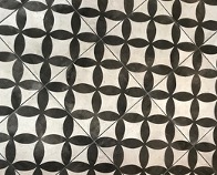
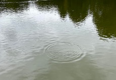
Just as we did with triangles, with circles we can think about angles formed inside them and their area and perimeter (circumference). Let’s begin with angles, and circle theorems, which are, in a way, a little like ‘the trigonometry of circles’.
3.8.1 Circle theorems
I sometimes begin by asking learners the following question:
What kind of triangle do you think will fit exactly inside a circle?
By ‘exactly inside’ I mean having all three of its vertices lying on the circumference of the circle.
Learners often suggest equilateral triangles, or triangles with three similar-sized angles, but in fact all triangles can be inscribed in a circle, as we will see later. This is not true for quadrilaterals - cyclic quadrilaterals are a specific category of quadrilaterals. A quadrilateral is cyclic if and only if its opposite pairs of angles sum to \(180{^\circ}\), as we will also see later. Otherwise, no circle can pass through all four of its vertices (Figure 3.70).

3.8.1.1 Paper folding
As we have seen, in contrast to quadrilaterals, all triangles can be contained inside a circle. One way to get a feel for this is to quickly (and not too carefully) cut out a lot of different acute-angled triangles from paper and give one to each learner. (Use a guillotine, to ensure that all the sides are straight, but don’t worry about the exact lengths or angles.) Ask them to fold perpendicular bisectors of each side by folding pairs of vertices onto each other (Figure 3.71).

The fold lines are equidistant from each pair of vertices. Where the fold lines intersect each other, therefore, must be a point that is equidistant from all three vertices, and this is called the circumcentre of the triangle. It follows that the three perpendicular bisectors of any triangle have to be concurrent - i.e. all pass through a common point. If we make this point the centre of a circle passing through any one of the vertices, the circle must necessarily pass through the other two, and therefore be the circumcircle of the triangle (Figure 3.72).

3.8.1.2 The angle at the centre is twice the angle at the circumference
If we make a triangle that has two vertices on the circumference and one at the centre, we discover that this has to be an isosceles triangle, because the two sides that join the circumference to the centre both have to be radii, and therefore must be equal to each other. This is using the key fact about a circle that every point on its circumference is the same distance from its centre.
Now, we can use the fact that the exterior angle of a triangle is equal to the sum of the two opposite interior angles (see Section 3.7.1) to find our first circle theorem.
In Figure 3.73, this means that the black angle at the centre of the circle must be the sum of the two grey angles. Since the two grey angles are equal to each other (since the triangle has to be isosceles), the black angle is twice either grey angle. The angle at the centre of the circle is twice the angle at the circumference, and this will be true however we move the two vertices on the circumference, as dynamic geometry can demonstrate.

We can put two triangles like this together. Although they are both isosceles, they do not have to be congruent; in fact, we can make the new triangle obtuse-angled if we wish, as shown in Figure 3.74.

In Figure 3.74, by the same logic, the white angle at the centre must be equal to the sum of the two light grey angles. Putting all of this together, the sum of the black and white angles must be twice the sum of one light grey angle and one dark grey angle. We could remove some of the ‘working’ and summarise it as in Figure 3.75: The angle subtended by an arc at the centre is twice that subtended by the same arc at the circumference.

We can use dynamic geometry to move the point on the circumference anywhere we like around the major arc, and although the angles at the other two vertices on the circumference will change, the angle we are moving doesn’t change, and neither does the angle at the centre. This is the theorem that angles in the same segment are equal.
If you have access to circular filter papers from the science department, these can be ideal for paper folding, because cutting out circles with scissors is time consuming and very difficult to do accurately enough. If all the filter papers are of equal size, different learners can draw the same length segment (e.g. \(5\) cm), but fold triangles from this segment to different positions on the circumference. All learners’ angles should be equal, and any two of the folded triangles’ angles should exactly fit together to make the angle at the centre (Figure 3.76).

Everything else derives from this first observation. Once we see how to use the exterior angle of a triangle to link what is happening at the centre of the circle with what is happening at the circumference, we can derive all the other circle theorems. We can even ignore all of the other circle theorems, and just use this one theorem every time, which is a little longer but involves less remembering!
3.8.1.3 Thales’ Theorem
You might recall with the triangle-folding activity that I advised ensuring that all the cut-out triangles were acute-angled. Learners could try the same task with a right-angled triangle, and they will discover that the circumcentre seems to land exactly at the midpoint of the hypotenuse (Figure 3.77) (Thales’ Theorem).

We can account for this by seeing it as a special case of our circle theorem, in which the angle at the centre is straight and the angle at the circumference (the ‘angle in a semicircle’) is therefore half of this, which is a right angle.
We can demonstrate the converse of this, which is also true, by drawing a circle and then putting the right-angled corner of a piece of paper onto the circumference. Where the edges of the paper meet the circle will always define a diameter (dashed line segment in Figure 3.78).

A nice way to use symmetry to prove Thales’ Theorem is to use a pair of perpendicular lines passing through the centre of a circle to partition the circumference into four equal arcs.
In Figure 3.79(a), I have marked one pair of arcs dotted and the other pair solid. If we now slide the vertical line some way to the right, the total length of the two solid arcs remains the same, as does the total length of the two dotted arcs (Figure 3.79(b)). This is because the portion of solid arc lost at the top is identical to the portion of solid arc gained at the bottom, by symmetry.
Similarly, if we slide the horizontal line upwards, again the total dotted length of arc and the total solid length of arc remain constant, and equal to each other, as they were in the original configuration, for the same reason. We can choose to slide both lines until they meet each other on the circumference (Figure 3.79(c)). Here, since the dotted arc and the solid arc must be equal, then each of them must be a semicircular arc, meaning that the right angle is the angle in a semicircle.

A memorable, physical way to appreciate Thales’ Theorem is to have learners stand along a large semicircle, such as by using the markings on a football pitch (Figure 3.80).

Ask everyone to face one end of the diameter and then close their eyes. Then each person is asked to turn themselves through \(90{^\circ}\) (in the correct direction), using the position of their feet to feel when they think they have rotated through \(90{^\circ}\). Finally, they open their eyes, and (with luck) they are all facing the other end of the diameter (Figure 3.81)!62

3.8.1.4 Circumcentre and incentre
For obtuse-angled triangles, the circumcentre does not lie within the interior of the circle. This makes it a little problematic when doing the paper folding, but once learners have got this far they can experiment with this case too.
They will find that their three fold lines head off, converging, but not to a point within the triangle. If they glue their triangle onto a larger sheet of paper, they can locate this centre, and use their compasses to verify that a circle centred there will indeed pass through all three vertices (Figure 3.82).

Playing slowly with dynamic geometry software, varying the positions of the vertices of the triangle and seeing how the circumcentre and circumcircle move is a great way to summarise all of this. Alternatively, keep the circle fixed and slide the triangle vertices around its circumference, looking at how the triangle changes shape.
It is possible to paper-fold angle bisectors of triangles, too. To do this, we have to fold the side edges, rather than the vertices, onto each other, for each pair of sides. These angle bisectors are equidistant from each edge (rather than from each vertex), and where these three lines meet is the point which is equidistant from all three sides.
There is no problem this time about the lines meeting off the paper – the incentre (as it is called) always lies within the interior of the triangle. A circle centred on the incentre can meet each side at a tangent, producing the inscribed circle of the triangle (Figure 3.83).

3.8.1.5 Tangent and radius
The only other necessary fact to know about angles and circles is that where a tangent meets a radius on the circumference, they always create a right angle.
‘Tangent’ is the same word from trigonometry, and means a line that meets the circle at a single point. (The triangle sides in Figure 3.83 are tangents to the inscribed circle.) A straight line can meet a circle \(0\), \(1\) or \(2\) times (Figure 3.84).

We can do a very informal kind of proof by contradiction that a radius and a tangent meet at right angles, by saying that if it were not the case that these lines met at right angles, then the angle on one side would have to be less than \(90{^\circ}\). Since the diagram is perfectly symmetrical, with nothing to distinguish one side over the other, we could argue exactly the same for the angle on the other side. But they cannot both be less than \(90{^\circ}\), since they must sum to \(180{^\circ}\), so our supposition that the lines did not meet at right angles must have been false. This basic idea can be sharpened up into a proper proof if desired, but it captures the essential idea.
3.8.1.6 Geoboards
A nice way to explore angles within circles is to use a \(12\)-pin geoboard - analogous to an analogue clockface - with \(12\) dots spaced evenly around the circumference (Figure 3.85).

Find all the different triangles that can be made by joining any three points on the circumference of a \(12\)-pin geoboard.
Calculate all the angles in each of the triangles you find.
By being systematic, learners should find the \(12\) triangles shown in Figure 3.86.

The angles in all of these triangles can be calculated by drawing in radii and finding isosceles triangles.
Without loss of generality, we can always have one vertex at the ‘\(12\) o’clock’ position, and therefore each triangle can be conveniently described by specifying the two ‘hours’ for the other two vertices (e.g. \(1\)-\(2\) for the first triangle, \(1\)-\(3\) for the second). This numbering can be helpful in ensuring learners go systematically through all of the possibilities.
3.8.2 Circumference and area
3.8.2.1 Circumference
Finally in our journey through circles, let’s look at perimeter and area, and begin with perimeter (i.e. circumference).
It is easy to overlook that this is a big deal. Learners will never have accurately measured the length of any curve before – and what does it even mean to measure ‘the length of a curve’? Learners may be used to the idea that length is how far along a ruler something goes, which is fine for straight lengths and straight rulers.
It is possible nowadays to get bendy plastic rulers, and they can be useful here, as can tape measures. Failing that, we can wind some string or thread along the curve, and then pull it straight and put it against the scale of an ordinary ruler. I don’t think anything more formal than this is needed at school level.
The main question to ask is, “How long is a circle?”63
In particular, we can ask:
Which is further - running all the way around the circumference of a circle, or running forward and back in a straight line through the centre - or are they the same?

If you have a large circle somewhere nearby, you could possibly do this for real. The centre circle of a marked football pitch is perfect for this (Figure 3.80).
With a moment’s thought, and perhaps by trying it out, it will be obvious to learners that it is much quicker to run back and forth along the straight line than to go all the way around the circumference.
There are some modelling assumptions here worth mentioning (Chapter 5): we assume that people run at constant speed, and we ignore any time taken to change direction at the end of the diameter. To avoid these, we could clarify that we are talking about the total distance run, rather than the time taken to run. Alternatively, you could perhaps imagine a light beam reflecting off the far end of the diameter, rather than a person running, if that helps to get away from the practical difficulties in the comparison.
Now, the task is to write down an inequality involving circumference \(c\) and diameter \(d\), which will be \(c > 2d\), or \(2d < c\).
We are supposing here that all circles are essentially ‘the same’ as each other, and what we discover by thinking about any ‘general’ circle will always apply. For instance, a circle with \(10\) times the diameter will have \(10\) times the circumference, otherwise it would not be the same shape. So, we can conclude that, no matter the size of a circle, its circumference will always be more than twice its diameter.
It may not be obvious to learners that we should expect the circumference of any circle to be the same constant multiple of its diameter. This is yet another example of thinking multiplicatively (Chapter 1), where we are seeking to find the magic multiplier that takes a diameter to a circumference:
\[ \begin{matrix} \text{diameter} & \fixedarrow{$\times \ ?$} & \text{circumference.} \\ \end{matrix} \]
Our inequality \(2d < c\) gives us some idea of the length of a circle, indicating a multiplier greater than \(2\), but can we do better?
Next, we might try comparing a circle inscribed within a square:
Which is further - running all the way around the circumference of a circle or running around the smallest square that the circle just fits inside - or are they the same?

This time, the circle wins over the square, because the circle ‘cuts the corners’ of the square. No one would want to have to run in and out of the corners of the square if they could just continue on the circle instead.
So, this time, \(c < 4d\).
We can combine what we have learned so far, by writing a double inequality:
\[2d < c < 4d .\]
The circumference is somewhere between \(2\) diameters and \(4\) diameters long. It looks very much as though \(c = 3d\) is going to be the answer.
We can investigate this by doing one final comparison, this time with a regular hexagon. Notice that while the square enclosed the circle, this time the circle encloses the hexagon:
Which is further - running all the way around the circumference of a circle or running around the smallest regular hexagon that just fits inside it - or are they the same?

Clearly, the hexagon is shorter than the circle here, because when making the journey between adjacent vertices of the hexagon we are faced with the choice of a straight line (along the hexagon) or a curve (along the circle). A straight line between two fixed points is always shorter than any curve. It is worth getting learners to articulate their reasoning precisely like this, rather than just all agreeing, “Yeah, that looks shorter”.
This time, finding an inequality linking circumference \(c\) and diameter \(d\) is a little trickier. By joining opposite vertices with diameters, we can see that a diameter is \(2\) hexagon edges. This means that the \(6\) edges of the entire hexagon must be \(3\) diameters, and that this is less than \(c\). This gives us \(3d < c\).
Putting all of these inequalities together, we get
\[2d < 3d < c < 4d .\]
Our first bit of reasoning with the double diameter that gave us \(2d < c\) is redundant, now that we have the tighter inequality from the hexagon that gave us \(3d < c\). We didn’t need to do any of this thinking to realise that \(2d < 3d\).
So, our conclusion is
\[3d < c < 4d .\]
This tells us we were wrong to guess \(c = 3d\), and in fact we can now see that the circumference cannot be an integer number of diameters, because there are no integers available between \(3\) and \(4\). The multiplier we are looking for must be some number between \(3\) and \(4\).
We could estimate this number by doing some measurements of circular objects, or we could just tell learners that the number is \(\pi = 3.14159\ldots\) and that not only is it not an integer, it is not even rational. Like the surds (\(\sqrt{2}\), etc.), it is irrational (Chapter 2).
Notice this means that if \(c\) is rational then \(d\) isn’t, and vice versa. They can both be irrational, but they can’t both be rational. When we say that \(\pi\) is the ‘ratio’ of the circumference to the diameter of a circle, we have to remember that the ‘ratio’ is not a ‘rational’ ratio.
Despite being told that \(\pi\) is irrational, learners will often happily write \(\pi = 3.14\). I have heard learners say that they appreciate that \(\pi\) ‘cannot be a fraction’, and therefore they assume that ‘it must be a decimal’. Of course, any terminating decimal, such as \(3.14\), is just as rational as any fraction, because we can always express it as an integer number of the final decimal place (e.g. here \(\frac{314}{100}\)). So, writing \(\pi = 3.14\) is just as problematic as writing \(\pi = \frac{22}{7}\). Indeed, \(3.14\) is actually a little further away from \(\pi\) than \(\frac{22}{7}\) is. By writing \(\pi = 3.14\ldots\), we can avoid implying that \(\pi\) has become rational.
Learners need to get used to using the \(\pi\) button on their calculator, which, while also an approximation of course, they can think of as containing the pure, exact value. Alternatively, it is usually most mathematical to just express answers in terms of multiples of \(\pi\), without doing an approximate decimal conversion.
This might seem like a lot of discussion, compared with just telling learners that there is a formula, \(c = \pi d\) or \(c = 2\pi r\), and letting them practise substituting in numbers. Couldn’t we have done this in Chapter 1 as an example of thinking multiplicatively? The trouble with this kind of approach is that it becomes ‘just another formula’. Being able to substitute numbers into formulae is an important skill in algebra, but here I would want the focus to be on the geometry of circles.
The linear relationship between diameter and circumference can be quite unintuitive.
Consider this task:
Imagine a pipe running along the surface of the earth, exactly along the equator.
(Don’t worry about the practicalities or the sea!)
How much longer would the pipe need to be if instead it were suspended \(1\) m above the surface of the earth, all the way round?
Learners may say they need to know the radius of the earth to work this out, but actually they don’t. However, you could provide it (about \(6,400\) km), or just say that you don’t recall it, and ask them to use the letter \(r\) and ‘substitute it in later’.
If we do this, where \(r\) is the radius of the earth in metres, then if we assume that the equator is a perfect circle, then the increase in length will be
\[2\pi(r + 1) - 2\pi r = 2\pi .\]
So, the extra pipe length needed would be only \(2\pi\) metres, or about \(6.3\) m, which seems hardly anything, relative to the huge circumference of the earth.
This is quite counterintuitive. One way to make it less so is to imagine that the earth were a cube instead, and so the ‘equator’ would be a square, rather than a circle.
When we move out the perimeter of the square by \(1\) m on each side, the four sides all retain their length, and the only length we gain is four quadrants (quarter circles) of radius \(1\) m at the four corners, shown dotted in Figure 3.87, which add up to \(2\pi\).

If we try a regular polygon with more sides, say a hexagon (\(6\)-gon), we find the same result. The only increase to the perimeter consists of the six \(\dfrac{1}{6}\)-turn additions, one at each vertex, each of radius \(1\) m, which together sum to a full circle, of length \(2\pi\) metres, as shown in Figure 3.88.

If we think of a circle as the limit of a regular \(n\)-gon, as \(n \rightarrow \infty\), then we have to imagine this extra circle of radius \(1\) m, with a length of \(2\pi\), being ‘smeared out’ all the way around the pipeline, as infinitely many infinitesimally small pieces. If we collected them together at one place, so we could see them, we would get a small additional arc, shown dotted in Figure 3.89.

Learners may enjoy this riddle:
I went on a journey and my head travelled \(12\) metres further than my feet did.
Where did I go?
The person went once around the world (upright, not lying down!), and their height was \(\displaystyle \dfrac{12}{2\pi} = 1.9\) metres.
Once learners master the idea of \(c = \pi d\), there is no need to explicitly teach that the semicircular arc length is half of this, or give a formula such as
\[\text{length of semicircle} = \pi r .\]
Any fraction of a circumference will just be the same fraction of \(\pi d\), so if learners are confident at thinking multiplicatively (Chapter 1), finding the length of a \(100{^\circ}\) arc of a circle, say, will be no problem. The multiplier will just be \(\displaystyle \dfrac{100}{360}\).
The only tricky thing with calculating a perimeter of a sector might be to remember to include the two radii, which are the straight parts of the perimeter.64
There are no other curve lengths that learners will be able to find exactly until they study calculus. Finding the length of a parabolic arc or a (non-circular) ellipse, for instance, is a considerably greater challenge.
For example, the length of the simple curve \(y = x^{2}\) from \((0,\ 0)\) to \((1,\ 1)\) turns out to be the complicated value \[\dfrac{2\sqrt{5} + \ln\left( 2 + \sqrt{5} \right)}{4} ,\]
and in general there is no nice formula for the arc lengths of ellipses – you just have to approximate the value numerically.
3.8.2.2 Area
Moving on to area, it might seem that we will have to do something similar to our approach to circumference in order to find a formula for the area of a circle (disc). But actually we can do this fairly easily by imagining dividing the circle into a large number of equal sectors.
We’ll begin with \(8\) sectors, which is not a very large number, so that we can see what we are doing more clearly. Then, we will imagine the same process with \(16\) or \(100\) sectors.
If we dissect our circle into, say, \(8\) equal sectors, and rotate every other one, we get an arrangement like that shown in Figure 3.90.

Doing the same thing with \(16\) sectors, and then \(100\) sectors, give the arrangements shown in Figure 3.91 and Figure 3.92. Using an app, you can experiment with other numbers of sectors and see the result.65


It looks as though we could approximate this shape as a parallelogram, and that the approximation ought to improve as we use more sectors. Eventually, with say \(1000\) sectors, you would be unable to tell that there was ever a circle to begin with. The little bumpy arcs along the top and the bottom would be hardly discernible any more, and the edges would appear straight.
In Figure 3.92, half of \(c\) is along the top, with the other half along the bottom, and the perpendicular height is roughly \(r\). Half of \(c\) is \(\pi r\), because this is half of \(2\pi r\), or half of \(\pi d\), because \(d = 2r\).
This leads to the result that the area of the original circle must be
\[\text{base} \times \text{height} = \pi r \times r = \pi r^{2} .\]
This is one of those famous formulae in mathematics, like \(E = mc^{2}\) in physics, so it is nice to make a bit of a fuss about it.
It turns out that if we split up our circle into ‘infinitely many’ sectors, the error in the approximation would disappear, and the formula would become exactly true. It is worth mentioning that we have assumed throughout that when you chop up a shape and reassemble the pieces, provided there are no gaps or overlaps, then the total area doesn’t change, and this is a perfectly reasonable assumption in school mathematics.66
Again, if learners have really appreciated what is going on here, then there is little more to say when it comes to finding areas of sectors. It is just thinking multiplicatively again (Chapter 1) to find the multiplier to apply to \(\pi r^{2}\), and this is all that is needed to work with pie charts in statistics (Chapter 1).
It is clear from the derivation that \(\pi r^{2}\) means \(\pi r \times r\), and not \((\pi r)^{2}\). Teachers sometimes teach the formula as \(r \times r \times \pi\), so as to avoid this possible confusion. But I think of this as not supporting learners’ familiarity with how algebra is conventionally written, and it seems a missed opportunity for reviewing the priority of operations (Chapter 2).
3.9 What does thinking geometrically get us?
Tony Gardiner has commented that:
The material of school geometry captures the spirit of mathematics better than almost any other part of elementary mathematics … All pupils can calculate some surprising things, can solve some interesting problems, and can prove some strikingly useful results; and more confident pupils can prove a wide range of remarkable and unexpected facts.67
I think this encapsulates very well the opportunities provided by geometry for ‘being mathematical’. A very small number of known geometrical theorems provide access to many rich and often quite difficult problems, as we will see in this section.
3.9.1 Bearings
Three-digit bearings, measured clockwise from North, can provide good opportunities to develop learners’ ideas of angle.
To practise the general idea, without worrying about accurate calculations, the teacher can define a ‘North’ direction in the classroom, and then ask learners to estimate the bearing of one learner from another (both ways round). Learners should develop the habit of estimating the approximate size of a bearing before measuring or calculating – they should at least know which multiple of \(90{^\circ}\) it is going to be closest to.
Coordinate grids are very useful in this context.
If we say that the positive \(y\) axis is North, then learners can choose any two integer points \(A\) and \(B\) on a \(- 10 \leq x \leq 10\) and \(- 10 \leq y \leq 10\) grid and measure the bearing of \(A\) from \(B\), and the back bearing of \(B\) from \(A\).
For example, they might choose \(A(5,\ 5)\) and \(B(2, - 2)\), and, in Figure 3.93, the bearing of \(A\) from \(B\) is the grey angle (\(023{^\circ}\)), and the bearing of \(B\) from \(A\) is the white angle (\(203{^\circ}\)).

Learners will observe that, in this case,
\[\text{white} - \text{grey} = 203{^\circ} - 23{^\circ} = 180{^\circ} ,\]
and in general,
\[\left| \text{bearing} - \text{back-bearing} \right| = 180{^\circ},\]
which they can prove using alternate angles. (It is arbitrary which bearing we count as the back-bearing: white is grey’s back-bearing, and grey is white’s back-bearing.) Their measurements will not be perfectly accurate, but they should obtain a value close enough to \(180{^\circ}\) to suggest that this could be the true difference.
Learners who know about trigonometry will be able to calculate, rather than measure, the angles, using the \(\text{tan}^{- 1}\) function. Getting a general formula is tricky, because you have to think about which point is to the right and which to the left.
If \(A(x_{A},y_{A})\) and \(B(x_{B},y_{B})\) are two distinct points, then:
If \(x_{B} < x_{A}\), then the bearing of \(A\) from \(B\) is \(\tan^{- 1}\left(\displaystyle \dfrac{y_{A} - y_{B}}{x_{B} - x_{A}} \right) + 90{^\circ}.\)
If \(x_{B} > x_{A}\), then the bearing of \(A\) from \(B\) is \(\tan^{- 1}\left(\displaystyle \dfrac{y_{A} - y_{B}}{x_{B} - x_{A}} \right) + 270{^\circ}.\)
If \(x_{B} = x_{A}\), then if \(y_{B} < y_{A}\), the bearing of \(A\) from \(B\) is \(000{^\circ}\), and if \(y_{B} > y_{A}\), the bearing of \(A\) from \(B\) is \(180{^\circ}\).
It is possible to set up a spreadsheet that calculates the bearing between any two pairs of entered coordinates.68
Learners can practise bearings by making a code for their partner.
First, they spread out the letters of the alphabet haphazardly across the page (e.g. Figure 3.94).

Then, they form a message by writing down distances and bearings (e.g. “Go \(5\) cm on a bearing of \(035{^\circ},\ \ldots\)”), beginning at the bottom left corner of the rectangle, that moves from letter to letter, spelling out the message. Finally, they swap and decode each other’s messages.69
3.9.2 Symmetry
3.9.2.1 Symmetry in 2D
Many young learners will be familiar with folding a piece of paper in half, unfolding it, putting some paint on one half and refolding, to obtain a symmetrical pattern, such as a butterfly (Figure 3.95).

Paper folding can be a powerful way of confirming or disconfirming a line of symmetry. It can also be useful for developing learners’ visualisation and reasoning.
Here is an example task:
Imagine folding a rectangular sheet of paper (e.g. a sheet of newspaper) in half, and then in half again, folding at right angles to the first fold, so you end up with a folded sheet that is the same shape as the original rectangle.
Now imagine using a pair of scissors to snip off one of the corners, with a single straight cut.
Predict and explain what you could see when the sheet is unfolded.
Depending on which corner is snipped off, and at what angle, we may obtain a square or a non-square hole, but any hole we obtain must be a rhombus, because the length we make with our cut will be the length of all four sides of any central hole.
However, we may not obtain a hole at all (see Figure 3.96).

Learners can explore what happens when they make different folds and different kinds of cuts.
We do not do anything formal with symmetry at school level, and it is purely descriptive. Learners may notice that when a shape has two lines of symmetry those lines are always at right-angles to each other, and they may find it interesting to explore why, by trying to draw shapes for which this is not the case.70
Rotational symmetry is usually more difficult than line symmetry, partly because ‘no’ rotational symmetry conventionally corresponds to an order of rotational symmetry of \(1\), not zero.
The teacher could ask a question like “What does an upside down parallelogram look like?” (see Section 3.5). Really the answer depends on what kind of parallelogram and what orientation it begins in. Many learners will think that a rectangle in its standard orientation will look the same upside down, but that a non-rectangular parallelogram will ‘lean the other way’ (Figure 3.97).

They may need to cut out the shape and physically turn it to confirm that it won’t.
We can say that a non-rectangular parallelogram has order \(2\) rotational symmetry, and that a non-square rectangle (an oblong) has the same. And we can ask learners to find a shape with ‘order \(4\)’ rotational symmetry and explain why it is order \(4\), rather than order \(2\). Getting learners to construct examples, rather than providing them, forces them to think more deeply about what kinds of shapes will or will not work.71
A square is the most obvious example of an order-\(4\) polygon, but there are others, such as the \(12\)-gon or \(8\)-gon shown in Figure 3.98.

Each of these shapes also has four lines of symmetry, but is that necessary for an order-\(4\) shape?
Looking at what combinations of symmetries are possible and impossible can be very interesting, simultaneously providing lots of practice at classifying shapes. The task in Figure 3.99 works well when printed onto a large sheet of paper for learners to collaborate on in pairs.72

Learners will realise that some of these cells are impossible, and the teacher might find it useful to recall that the only finite symmetry groups in \(\mathbb{R}^{2}\) are \(Z_{n}\) (the cyclic group), along the top row, which have rotational symmetry but no line symmetry, and \(D_{n}\) (the dihedral group), down the diagonal (after \(D_{1}\)), which have both.
Learners will appreciate that these shape families extend beyond the limits of this table, and they often query where a circle would fit in. A circle has infinitely many lines of symmetry and an infinite order of rotational symmetry (and belongs to the orthogonal group \(O(2)\)).
Awareness of symmetry cuts across algebra, geometry, functions and graphs, and is a deep idea in mathematics. We will examine transformations in Chapter 4.
3.9.2.2 Symmetry in 3D
Symmetry of 3D shapes can be extremely difficult.
For example, a cube has \(9\) planes of symmetry: \(3\) parallel to the faces (fairly easy to imagine) and \(6\) at \(45{^\circ}\) angles to pairs of faces (much harder to imagine).
A non-cube square cuboid (i.e. a cuboid which is not a cube but has a pair of square faces) has a total of \(5\) planes of symmetry, and a non-square cuboid has just \(3\) (the ones parallel to the faces) (Figure 3.100).

A cube also has \(13\) axes of rotational symmetry, which are tricky to visualise. There are \(3\) through the centres of opposite faces, \(4\) through pairs of opposite vertices and \(6\) through the mid-points of opposite edges.
But some questions in 3D are easier than they might seem. For example, a cube has face diagonals, between the opposite vertices of the same face, and space diagonals, between opposite vertices that do not share a common face. A question that may seem difficult is:
What is angle between two face diagonals on a cube?
It can be hard to visualise the required angle.
However, if three face diagonals are draw to create a triangle (Figure 3.101), then it is clear that, by symmetry, the sides of the triangle must be the same length as each other (since the shape is a cube), and therefore that the triangle is equilateral. This means all of the angles are \(60{^\circ}\).

Learners may be surprised that you can slice a flat plane through a cube and get an equilateral triangle (Figure 3.102).

They may also be surprised that a plane parallel to this plane, but passing through the midpoints of the edges of the cube, can reveal a regular hexagon (Figure 3.103). It is also true that if you rotate a cube in front of a light source, to just the right orientation, its shadow can be a regular hexagon.

3.9.3 Plans and elevations
Plans and elevations have obvious real-life applications to building designs and putting together self-assembly furniture. The topic also lends itself well to puzzles, such as this:
The drawings below show two elevations and a plan view of an object.
Try to build this object using cubes.

How many possible different objects are there?
What is the smallest number of cubes necessary?
What is the largest possible number of cubes that could be used?
Make up a task like this of your own.
Learners can be asked to make up similar puzzles for each other, say using \(5\) given cubes to make any pentacube, and this can generate a lot of useful practice. There are \(29\) distinct pentacubes, so there are plenty of possibilities, and some of these are quite difficult.
For objects like these, plans and elevations are usually drawn on squared paper, whereas the object itself is easier to represent on isometric paper, as shown in Figure 3.104.

An interesting exercise is to give a learner a polycube (e.g. a pentacube or hexacube) inside an opaque bag (or even inside a sock) and ask them to sketch it on isometric paper, just by feeling the polycube, without removing it from the bag or looking inside.
I know of no better way to develop these skills than to use the Wisweb widgets,73 which can help learners develop their visualisation and mental rotation skills.74
3.9.4 Nets
Not all familiar everyday solids have a net. In particular, a sphere doesn’t, as anyone will know who has ever tried to wrap up a football as a birthday present! There are cross-curricular links here with geography, and the challenges and choices involved in making a flat map of the earth.75
Learners may be puzzled that cones and cylinders, like spheres, also have curved surfaces, but do have nets. They will have made cylinders by rolling up a flat piece of paper, and similarly for cones, and may have wondered why they can’t make a sphere from a flat piece of paper - other than by screwing it up into a ball!
There are different kinds of curvature involved here. A cylinder or the curved surface of a cone have zero Gaussian curvature, the same as a flat piece of paper, whereas a sphere has a constant positive Gaussian curvature - larger, the smaller the sphere.
There are many ambiguities associated with 3D shapes. Sometimes, it is not even obvious whether a drawing is intended to be 3-dimensional or not. For example, does Figure 3.105 represent a regular hexagon divided into three congruent rhombuses (2D) or a cube (3D)?

Just as, strictly, a ‘circle’ refers to the \(1\)-dimensional curve, and the interior can be termed a ‘disc’, we have similar terminology with ‘sphere’ (the 2D surface) versus ‘ball’ (the 3D shape). These can be very difficult to illustrate in printed diagrams on paper. Digital tools are useful, but a box of wooden (or clear plastic) 3D shapes is invaluable.
Drawing nets for a variety of different shapes may be interesting.76

Of the \(35\) possible hexominoes (Figure 3.106), only \(11\) are nets of a cube, and it can be a good task for learners to find all of them systematically (Figure 3.107).

The most common cubes to find in a mathematics lesson are dice, and most dice follow the rule that the sum of pairs of opposite faces is a constant. For a standard \(1\)-\(6\) die, this means that pairs of opposite faces will sum to \(7\). It follows from this that only one of the two dice shown in Figure 3.108 could be of this kind.

On the die on the left, we can see that the \(2\) and \(5\) faces are adjacent, and therefore cannot be opposite each other. The die on the right could be a standard die, but it depends on how the other three unseen faces are marked.
It turns out there are two distinct ways to make a standard die: left-handed and right-handed (Figure 3.109).

Because of the orientation of the pips on each face, it is sometimes possible to tell that two standard dice of the same handedness cannot be identical to each other. For example, in Figure 3.110 we can deduce that both dice could be standard right-handed dice, but they cannot be physically the same die because of the positioning of the pips on the \(3\)-face. The relationship between the direction that the \(3\) pips are going in and the \(1\)-face is different in the two dice. This can be less obvious when the dice are not viewed in the same orientation.

Learners can work on their visualisation skills by trying puzzles such as TASK 3.21 and inventing similar ones for their partner.
The net shown below is folded up to make a cube.
Which symbol will the finger point to?

The answer is the heart.
Working with 3D shapes can be a lot of fun, and learners will enjoy designing nets for various 3D shapes and seeing if they do actually fold up to make the desired shape. It is easy to learn about what works by trying different things. When designing nets, there are also opportunities for estimation and use of trigonometry or Pythagoras’ Theorem, depending on the complexity of the intended shape.77
A nice project relating to this is the following:78
Design a shape sorter for a young child, to help with their development of spatial knowledge.
Ideally, each shape, however you rotate it, will go through only one hole, so as not to confuse the child.
As an additional constraint, to help with tidying away, all the shapes should fit nicely inside the box.

It is possible to make this task quite simple or quite demanding, as you wish. For example, a nice challenge is to use only cuboids for all the shapes, which might initially sound impossible, but isn’t.
A nice task for calculating with nets and applying Pythagoras’ Theorem is the following (but adapt if anyone is arachnophobic):79
Imagine there is a spider in the back top left corner of the room shown below.
Suppose it wants to get to the very opposite corner, at the bottom right front.
What is the shortest route it can take?

A fly could take the space diagonal and, as that is the straight line that joins the two points, it must be the shortest possible route. But spiders can’t fly. So, if the spider must crawl along the surfaces, what is the shortest route it can take?
We could suppose the room is a cuboid, with horizontal dimensions \(5\) m by \(6\) m, and is \(3\) m tall.
Then the fly’s distance would be \[\sqrt{3^{2} + 5^{2} + 6^{2}} = \sqrt{70} \text{ metres},\] which is \(8.37\) m, correct to \(2\) decimal places.
Learners might know ‘Pythagoras’ Theorem in 3D’ as \(a^{2} + b^{2} + c^{2} = d^{2}\), or they might reason, using 2D Pythagoras’ Theorem twice, that the face diagonal of the base in the figure in TASK 3.23 will be \(\sqrt{a^{2} + b^{2}}\), and so the space diagonal we require will be
\[\sqrt{\left( \sqrt{a^{2} + b^{2}} \right)^{2} + c^{2}} ,\]
which is equivalent to \(\sqrt{a^{2} + b^{2} + c^{2}}\).
The spider’s distance is bound to be longer than this, but what is the shortest it can be?
Learners are likely to try routes such as those shown in Figure 3.111, using three different face diagonals.

If they are working with the values \(a = 5\), \(b = 6\) and \(c = 3\), they may be surprised that the total distances do not come out to be equal. They will obtain the distances \(3 + \sqrt{61}\), \(5 + \sqrt{45}\) and \(6 + \sqrt{34}\) which, correct to \(2\) decimal places, are \(10.81\) m, \(11.71\) m and \(11.83\) m. All of these are necessarily longer than the space diagonal a fly could take, which was \(8.37\) m.
Why does using the face diagonal of the face \(ab\) lead to the shortest total distance in this case?
It is because \(a = 5\) and \(b = 6\) are the two largest dimensions, so we save the most by cutting across the face that has those dimensions. Whichever dimension is not part of the face we cut across contributes its full value (the \(+ c\), \(+ b\) or \(+ a\) in the expressions in Figure 3.111), so we want this to be the smallest of the three dimensions.
However, none of these is actually the shortest route possible.
If we unfold the cuboid into its net, we can find a shorter route, shown in Figure 3.112(a), which is a straight line on the net, and which doesn’t have the unnecessary constraint of passing through a vertex. This route avoids travelling along the entirety of any of the cuboid’s individual dimensions. The distance is \(\sqrt{5^{2} + 9^{2}} = \sqrt{106}\), which is \(10.30\) m.

And even this is not the shortest route possible. Figure 3.112(b) shows the shortest route there can be, which has length \(\sqrt{6^{2} + 8^{2}} = 10\) m.
Learners can generate lots of useful practice by experimenting to find the lengths of different routes for different values of \(a\), \(b\) and \(c\).
3.9.5 Volume and surface area
Informally, we can think of volume as the amount of empty space inside a hollow object, the amount of liquid a closed hollow object could contain (its capacity) and the amount of liquid a solid object could displace – assuming the object does not dissolve or absorb the liquid when placed in it.
In a similar informal way, we can liken the surface area of a 3D object, or the area of a 2D object, to the quantity of paint it would take to cover its surface. The length of a 1D line is then the amount of ink it would take to draw that line.
However, there are many ambiguities which come into play in \(3\) dimensions.
For example, the surface area of a sphere would be just the outside, since if we dipped it into a pot of paint, only the outside would become covered. Similarly, the surface area of a closed cone (whether solid or ‘full of air’) includes the disc that is its base, as well as the curved surface on the outside. However, an open cone would get coated on the inside as well, so should should the surface area include this part too (see Figure 3.113)? Without more information, or a meaningful context, what is intended may be ambiguous.

Similarly, it matters whether a cylinder comes with discs at one or both ends, or is completely open.80
Alternatively, if surface area is defined as the area of an object’s net, then this would presumably only include one side of the net.
It is important to make learners aware of these complications, so they do not have to think about them for the first time when trying to interpret the possible meaning of a high-stakes examination question.
It is possible to justify formulae such as those for the volume of a cone and a sphere, but not very easily at this level.81 All of this is much more insightful to do when studying calculus, but for pre-calculus it feels to me a bit of a dead end, and can descend into merely substituting numbers into given formulae. For me, it is enough at this level to rely on demonstrations, such as peeling an orange and showing that the orange peel from an approximately spherical orange of radius \(r\) fits approximately into four copies of a disc of the same radius, to confirm the plausibility of the \(4\pi r^{2}\) formula. Of course, it is important that learners are clear that this does not constitute a proof!
Learners can develop their facility calculating volumes through tasks such as the one below.82,83
Design a gold coin that is worth exactly \(£100\).
You need to give its exact dimensions.
Think about what dimensions would be sensible in practice for such a coin.
For an extra challenge, make a \(£100\) coin that has both a gold part and silver part.
Learners will need to be told, find out for themselves or estimate values such as the current price of gold and its density.
Length, area and volume scale factors are the multipliers that come into play when we compare an object with an enlarged version of itself.
If the linear (length) scale factor is \(m\), then the area scale factor is \(m^{2}\) and the volume scale factor is \(m^{3}\):

This can help to make sense of the confusing array of units that exist for areas and volumes.
Given that \(100 \text{ cm} = 1 \text{ m}\), learners will often assume that \(100 \text{ cm}^2 = 1 \text{ m}^2\) and \(100 \text{ cm}^3 = 1 \text{ m}^3\).
These cannot be right if we consider what sketches of these quantities would look like (Figure 3.114).

Knowing how different quantities scale with size is very powerful.
One way into this is to ask learners the following question:
Imagine you woke up this morning and everything had doubled in size.
Would you be able to tell?
At first, learners are likely to think it would be obvious – everything would look so much bigger you couldn’t miss the change! But what if your eyes were bigger too? Everything would be twice as far away, so maybe it would look the same. You might expect that if you were twice as tall you would bang your head on the doorframe of your bedroom, but remember that the doorframe is also twice as big.
The answer really depends on exactly what we mean by ‘doubled in size’ and ‘everything’.
If our linear dimensions increased to twice their length, our volume would increase by a factor of \(2^{3} = 8\).
If our density remained the same, our mass would become \(8\) times as great.
Would our legs be able to support us? They would be stronger too, but only proportional to their cross-sectional area, so about \(4\) times as strong.
That means the pressure in our bones would be \(\dfrac{8}{4} = 2\) times as much.
If an ant were scaled up to our size, its legs wouldn’t be able to support its weight. This is why large, heavy animals, like elephants have to have fat, thick legs.
The essay On Being the Right Size, by JBS Haldane, is a very short, accessible, and quite amusing read.84 He points out that gravity is nothing to fear if you are small enough. An insect will not be hurt by falling out of a window, even though the distance to the ground, relative to its size, is comparable to a human falling out of an aeroplane!
Haldane memorably puts it:
You can drop a mouse down a thousand-yard mine shaft; and, on arriving at the bottom it gets a slight shock and walks away, provided that the ground is fairly soft. A rat is killed, a man is broken, a horse splashes.
An animal that is \(10\) times the size of another will have \(10^{3} = 1000\) times as much weight, but only about \(10^{2} = 100\) times as much air resistance as it falls through the air. So, the terminal velocity it reaches when falling through air (when the air resistance has increased enough to exactly balance out the weight) will be considerably greater for larger animals. A mouse requires no parachute (Figure 3.115), but an elephant most definitely does.
These considerations also explain why babies need to be kept warm. Because they are small, the ratio of their surface area to their volume is much less than for an adult, so they lose their heat more quickly.
Other links to science include the design of the lungs to maximise their surface area and the way in which solids dissolve more quickly, and react faster, when ground into smaller particles, with a greater total surface area to come into contact with a liquid or gas.
Knowledge of scale factors also enables a very elegant proof of Pythagoras’ Theorem.85
Figure 3.116 shows three, similar right-angled triangles.

The two smaller ones, with hypotenuses \(a\) and \(b\), fit together exactly inside the largest one, which has hypotenuse \(c\). Such a diagram will be possible for any \(a\)-\(b\)-\(c\) right-angled triangle.
Angle chasing shows that the triangles are similar (AAA).
Since the areas of similar triangles are proportional to the square of any corresponding side,
- area of triangle with hypotenuse \(a = ma^{2}\)
- area of triangle with hypotenuse \(b = mb^{2}\)
- area of triangle with hypotenuse \(c = mc^{2}\),
all with the same multiplier \(m\) (constant of proportionality).
Since the \(a\)-triangle and the \(b\)-triangle fit exactly together inside the \(c\)-triangle, the areas must add up:
\[ma^{2} + mb^{2} = mc^{2}.\]
And, since \(m \neq 0\), we can cancel the \(m\)’s to obtain
\[a^{2} + b^{2} = c^{2} ,\]
which is Pythagoras’ Theorem (see Section 3.7.5.3).
3.10 Problem solving with thinking geometrically
There aren’t many important geometrical theorems in school mathematics. And yet, with a relatively small ‘bag of tricks’, learners can potentially solve an impressive array of often quite challenging problems.
There are many sources of challenging puzzles which require minimal knowledge of geometrical facts to solve, relying more on persistence and ingenuity.86 Algebra (Chapter 2) is sometimes necessary or helpful.
Carefully chosen problems can provide opportunities for learners to develop effective tactics for problem solving.87
I will focus in the problems below on just one particular tactic that sounds simple, but is highly versatile and extremely powerful: adding auxiliary lines. By auxiliary lines, I mean additional lines that are not present in the original problem, but which facilitate a solution.
We have already seen examples of using this tactic earlier in this chapter (e.g. in Section 3.7.1 and Section 3.7.3). As learners see, again and again, the power of adding such lines, they will become comfortable exercising their freedom to do so whenever they think it might be helpful. They will gradually become better able to make effective choices about which line to add, and when.
3.10.1 The ku angle problem
The problem below is widely used in Japanese mathematics lessons, and is referred to by the Japanese hiragana character “ku” (く), because this looks similar to the configuration of lines in the diagram.88
Find the size of angle \(x\) in the figure below.

Initially, learners can be quite stuck. However, an auxiliary line parallel to the horizontal lines and passing through the vertex containing \(x\) dramatically unlocks the problem, by creating two pairs of equal alternate angles (Figure 3.117).
Suddenly, it becomes clear that \(x = 50{^\circ} + 60{^\circ} = 110{^\circ}\).

By working on this problem, learners will discover that not all plausible-looking auxiliary lines are equally useful.
For example, the dashed line in Figure 3.118, joining the vertices on the parallel lines, does not instantly lead to a solution.

To make this auxiliary line work, we need to introduce a second unknown, \(y\).
Then we can note that interior angles on the parallel lines are supplementary, meaning that the unmarked angle in the triangle must be equal to
\[180{^\circ} - (60{^\circ} + y) - 50{^\circ} = 70{^\circ}-y .\] Now, we can set the sum of the angles in the triangle to \(180{^\circ}\): \[x + y + (70{^\circ}-y) = 180{^\circ} .\] So, \[x + 70{^\circ} = 180{^\circ} ,\] meaning that \(x = 110{^\circ}\), as before – but with a lot more fuss. This was not a good auxiliary line for this problem.
A third auxiliary line, shown in Figure 3.119, passes at right angles to the parallel lines, creating a quadrilateral in which we can easily find all the angles other than \(x\).

Using the fact that the interior angle sum of a quadrilateral is \(360{^\circ}\), we can find \(x\):
\[\begin{alignat*}{2} x & + (90^\circ - 50^\circ) + 90^\circ + (180^\circ - 60^\circ) &&= 360^\circ \\ x & + 250^\circ &&= 360^\circ \\ x & &&= 110^\circ \end{alignat*}\]
Even though this auxiliary line creates a polygon with more sides than the triangle created by the previous auxiliary line, it gives a quicker, much easier solution.
Choosing where to place an auxiliary line is a subtle matter that may require some trial and error. The point of using this problem with learners is not just to solve the problem and move on, but to get better at seeing how to select good auxiliary lines, and appreciating why less good auxiliary lines are less good.
We can extend this problem by adding more angles in between the parallel lines, changing the V shape into more of a reverse-Z shape:
Find the size of angle \(x\) in the figure below.

Here, two auxiliary lines are needed, and learners could invent problems which require three or more.
We have
\[x = 50{^\circ} + 110{^\circ} - 30{^\circ} = 130{^\circ} .\]
Learners can create related problems by finding the angles where two equiangular polygons overlap.
Here is an example:89
In the figure below, two equilateral triangles overlap.
The angle shown is \(20{^\circ}\).

Which other angles in the figure can you find?
In fact, all the missing angles in the figure can be found.
Learners can extend the problem by adding a third equilateral triangle or by incorporating other equiangular polygons, such as rectangles.
We can use the same kind of diagram to pose area problems too:
The white and grey areas in the figure below represent two people’s land.
The V-shaped line is the boundary between them.

The neighbours want to replace the V-shaped boundary with a single straight line, so they each retain the same amount of area as they have now.
How can they find where to put the new fence?
Again, the key is to introduce an auxiliary line, but where should it go?
The line we put in before (Figure 3.118), that was not very useful then, turns out to be ideal for this problem!
We join the vertices where the fence meets the parallel lines, and we construct a second auxiliary line parallel to this one and passing through the vertex in the V (Figure 3.120).

Now, we can slide the V vertex along this second auxiliary line, to either parallel line, to create the position for the new fence (Figure 3.121).

The amount of grey area must be constant, because both the base and the height of the grey triangle remain the same. And, if the grey area remains constant, the white area must do too.
Of course, the validity of this solution depends on assuming that all the land is uniform quality, and only the total area each person gets matters.
3.10.2 Tying a knot in a piece of paper
Take a long rectangular strip of paper.
Tie a very loose knot in it.
See if you can gradually tighten the knot, and flatten it down, to make a pentagon, as shown below.

Is it a regular pentagon?
It is definitely a pentagon, because it is a polygon with five sides. But it looks like a regular pentagon, and the task is to prove it is regular.
The folding creates equal angles and equal lengths, and we can use auxiliary lines to mark these and help us see what is going on.
We can see that the first fold creates a pair of equal angles (dark grey and black in Figure 3.122).

In Figure 3.123, the light grey angle and the dark grey angle are equal, because of the fold - they lie on top of each other when the paper is folded. The light grey angle and the black angle are also equal, because of alternate angles (the strip of paper has parallel edges). So, the dark grey and black angles are equal, and the fold creates an isosceles triangle.

By an identical argument, the second fold creates a second, congruent isosceles triangle, and the third fold creates a third one. The three isosceles triangles are shown in Figure 3.124, with the pair of equal angles marked in grey and the other angle marked in white. Two equal white angles (corresponding and alternate) are also included.

Looking at the three diagrams together, we can see that each vertex consists of one grey angle and one white angle, meaning that all five interior angles are equal. Using these equal angles, and the equal sides from the isosceles triangles, we can prove that all the sides of the pentagon are also equal.
We can also see that each grey angle is twice each white angle. Since two greys and a white make a triangle (\(180{^\circ}\)), each white angle must be \(\dfrac{180{^\circ}}{5} = 36{^\circ}\), so each grey angle is \(72{^\circ}\) and each interior angle of the pentagon is a grey plus a white, which is \(36{^\circ} + 72{^\circ} = 108{^\circ}\).
3.10.3 Standing in the garden
I am standing in a rectangular garden.
My distances from three of the corners are shown below (not drawn to scale).
How far am I from the fourth corner?

It may feel as though there is not enough information to solve this problem, but actually there is.
Learners might wonder whether it matters which corner is which - if we swapped around two of the given lengths, would it be the same problem or a different one? The answer is that it would be different.
Again, auxiliary lines come to the rescue.
An experienced problem solver might say, “It looks like a Pythagoras’ Theorem problem”, but a learner might object, “But there aren’t any right-angled triangles!” Although there are no right-angled triangles, there are right angles in the four corners of the rectangle. And if we place auxiliary lines judiciously, we can create some right-angled triangles, as in Figure 3.125.

Using the notation in Figure 3.125,
\[ \begin{alignedat}{2} 9^{2} - a^{2} &= {h_{1}}^{2} = x^{2} - b^{2} && \rlap{\qquad \text{①}} \\ 6^{2} - a^{2} &= {h_{2}}^{2} = 2^{2} - b^{2} && \rlap{\qquad \text{②}} \end{alignedat} \]
We can eliminate the \(a^{2}\) and the \(b^{2}\) by subtracting one equation from the other:
\[ \begin{alignedat}{2} 9^{2} - 6^{2} &= x^{2} - 2^{2}, && \rlap{\qquad \text{①} - \text{②}} \end{alignedat} \]
giving
\[ \begin{alignedat}{2} x^{2} &= 9^{2} - 6^{2} + 2^{2} = 49 . && \end{alignedat} \]
Taking the positive square root, since \(x\) is a length, gives \(x = 7\), so I must be \(7\) metres from the fourth corner.
Here, some algebra was a necessary part of the solution, and the problem is an application of the so-called British flag theorem.
A follow-up question might be to wonder when you will obtain integer solutions from a problem like this. What was it about the numbers \(2\), \(6\) and \(9\) (and their positions) that made the answer come out to be an integer? Put differently, where can you stand in the garden so your distances to every corner are an integer number of metres?
There is lots to explore here. To create this problem, I began with a number (\(85\)) which can be expressed as the sum of two squares in two different ways. The number \(85\) can be expressed as both \(2^{2} + 9^{2}\) and \(6^{2} + 7^{2}\), and this allowed me to devise a problem with an integer solution.
3.10.4 Getting under a rope
This is a nice, counterintuitive Pythagoras problem:
A string has length of \(101\) cm.
Its ends are attached to two screws fixed \(1\) m apart on flat ground, as shown below (not drawn to scale).
 The string is not stretchy.
What is the largest animal you think could pass underneath the string?
There is only \(1\) cm of ‘play’ in the string, so learners are likely to think of very small animals, such as a fly or a caterpillar. But there is much more space under the string than learners may expect.
If we imagine pulling the string as far up as it will go, midway between the screws, we get the diagram shown in Figure 3.126.

Using Pythagoras’ Theorem in either of the two congruent right-angled triangles, the maximum height \(h\) cm of the string will be given by
\[h = \sqrt{{50.5}^{2} - 50^{2}} = 7.09\text{ (correct to 2 decimal places)}.\]
The value of \(7.09\) cm is much greater than the \(1\) cm additional length of the string, and learners may be surprised that a difference as small as \(0.5\) cm in the numbers being squared can lead to such a large answer.
The height is large enough that a small cat could fit through this gap, since cats can generally get through any hole that is larger than their head.
We can generalise our expression for \(h\) to a horizontal distance of \(2x\) (more convenient than calling it \(x\)) and a string that is an amount \(2\delta\) longer than \(2x\).
In that case, we obtain
\[h = \sqrt{(x + \delta)^{2} - x^{2}} = \sqrt{x^{2} + 2x\delta + \delta^{2} - x^{2}} = \sqrt{2x\delta + \delta^{2}} .\]
If we assume that \(\delta\) is much smaller than \(x\), then we can approximate this.
If \(\delta \ll x\), then, to a first approximation, \(\delta^{2}\) will be negligible, and we can write
\[h \approx \sqrt{2x\delta} ,\]
and, when \(2x = 100\), this reduces to
\[h \approx 10\sqrt{\delta} .\]
This enables us to see why \(h \gg \delta\). With \(2\delta = 1\), we obtain \(h \approx 5\sqrt{2}\), which at \(7.07\)… is very close to the \(7.09\) cm value we calculated. It is a little low, because we threw away the \(\delta^{2}\) term.
3.10.5 The area of an annulus
Finding right-angled triangles, and therefore using Pythagoras’ Theorem, in unlikely situations, is a common theme. Auxiliary lines can often reveal a lurking right-angled triangle that enables a solution.
Consider this problem:
Express the area of the shaded annulus below in terms of \(x\).

An annulus is the region between two concentric circles (circles with a common centre).
It feels as though we do not have sufficient information to answer this question, because we have just one distance, \(x\), whereas there are two circles, with different, unknown radii.
We will assume that the dashed line is a tangent to the smaller circle.
If we add two auxiliary lines – the radii of both circles – we obtain a right-angled triangle (Figure 3.127).

We can then use Pythagoras’ Theorem to see that, if \(r\) is the radius of the smaller circle, and \(R\) is the radius of the larger circle, then
\[x^{2} = R^{2} - r^{2} .\]
If we multiply through by \(\pi\), we obtain
\[\pi x^{2} = \pi R^{2} - \pi r^{2} .\]
The right-hand side is the shaded area of the annulus, because is is the difference between the area of the large circle and the area of the small circle, and the equation tells us this is equal to \(\pi x^{2}\).
Although we don’t know the values of \(r\) and \(R\) separately, \(x^{2}\), which we do know, gives us the difference between their squares, which turns out to be exactly what we need to find the area.
One way to obtain the answer without using Pythagoras’ Theorem is to assume that the length \(x\) by itself is sufficient information to determine the area of the annulus. If this is true, then the precise areas of the circles cannot matter, and so we could vary the radii of both circles, and provided that \(x\) remained constant, the shaded area would not change (Figure 3.128).

If this is true, then we could, for convenience, imagine shrinking the smaller circle down to nothing at all, which would leave \(x\) equal to the radius of the larger, now completely shaded circle, whose area would now be \(\pi x^{2}\), as we found above. But this solution does require assuming that the shaded area depends on \(x\) only; i.e. that the problem contains sufficient information.
3.10.6 Dividing into thirds
This task tends to provoke a lot of thinking:90
Two people each wanted to divide a disc into thirds.
Their attempts are shown below.
What measurements could you make to see if they have done it correctly?

Most learners will agree with the division on the left but disagree with the one on the right.
However, in fact both have correctly divided the area of the disc into three equal regions, at least as accurately as it is possible to represent in these figures.
On the right, the areas of the three regions are the same, but the three pieces are clearly not congruent, as they are on the left. In addition, the circle (i.e. the circumference) on the right has clearly not been divided into three equal pieces.
Learners may assume that the figure on the right has been constructed by making two horizontal lines that divide the vertical diameter into three equal lengths. However, that is not the case. We can contrast dividing the diameter into three equal pieces (in Figure 3.129(a)) with dividing the area into three equal pieces (in Figure 3.129(b)), which is identical to the right-hand figure in TASK 3.34).

The impression in Figure 3.129(b) may be that the middle piece is smaller in area than each of the two outer pieces, but this is a visual illusion. It must be the case in Figure 3.129(a) that the middle piece has greater area than either of the outer pieces, because the circle is wider near its middle. Moving the horizontal lines to the positions in Figure 3.129(b) turns out to be just sufficient to make the three areas equal, but how can we confirm that this is the case?
As before, radii are the ideal auxiliary lines needed to do this.
By symmetry, we can focus on just the top region in Figure 3.129(b), and we just need to show that it is one-third of the area of the entire disc.
In Figure 3.130, I have joined both ends of the chord to the centre, \(O\), and marked the angle \(\theta\) at the centre.
If we take the circle as being a unit circle (i.e with a radius of \(1\)), then we can use \(\dfrac{1}{2}ab\sin\theta\) to find the area of the white triangle, which will be \(\dfrac{1}{2}\sin\theta\), since both \(a\) and \(b\) are the unit radius.

To find the grey area in Figure 3.130 (the segment), we need to subtract the area of the white triangle from the area of the sector.
The sector will have area \[\dfrac{\theta}{360{^\circ}}\pi r^{2} ,\]
but the radius \(r\) is equal to \(1\), so this reduces to \(\displaystyle \dfrac{\theta\pi}{360{^\circ}}\) , meaning that the grey area must be \[\dfrac{\theta\pi}{360{^\circ}} - \dfrac{1}{2}\sin\theta .\] We want this to be equal to one-third of the area of the circle, or \(\displaystyle \dfrac{\pi}{3}\), so
\[\dfrac{\theta\pi}{360{^\circ}} - \dfrac{1}{2}\sin\theta = \dfrac{\pi}{3} .\]
We can clear the fractions by multiplying through by \(360{^\circ}\) to give \[\theta\pi - 180{^\circ}\sin\theta = \pi \times 120{^\circ}\] \[(\theta - 120{^\circ})\pi = 180{^\circ}\sin{\theta}.\]
(This looks neater in radians, but I am assuming learners don’t yet know about radians.)
This is not an equation we can solve analytically, so we will need to use technology and/or trial and improvement to find a solution.
We obtain \(\theta = 149.27{^\circ}\), correct to \(2\) decimal places, so the white triangle is close to a \(15{^\circ}\text{-}15{^\circ}\text{-}150{^\circ}\) triangle. We can draw in the auxiliary radii and measure this angle in Figure 3.129(b) to confirm that the horizontal lines are indeed in approximately the correct positions.
3.10.7 Cutting a cake
A contrived but quite challenging problem is the following:91
Imagine a cylindrical cake, with its circumference marked into \(12\) equal arcs (like a clockface).
Someone wants to cut \(6\) slices of cake.
Instead of doing it in the obvious, conventional way, as shown on the left below, they decide to do it as shown on the right.

How similar are the sizes of the six pieces \(a\)-\(f\)?
Learners might begin by considering whether the pieces on the right in TASK 3.35 are of equal size.
They do not look as though they all are, but we can reason that \(c\) and \(f\) must have the same area as each other, since they are congruent segments.
It may be worth asking learners to try to order the pieces ‘by eye’ from smallest to largest area. Then, they can calculate to see how good their estimates were.
If we take the circle as having unit radius, we obtain the results given below.

Learners can compare this with the order they estimated by eye.
3.10.8 Pizza slices
This task can be useful for thinking about how length and area scale differently. It is not necessary for learners to know the formula \(\pi r^{2}\) for the area of a circle in order to access this.92
One evening, you order a \(20\)-inch pizza to be delivered.
The pizza company apologise and say they don’t have any \(20\)-inch pizzas.
But they will send you two \(10\)-inch pizzas instead.
Is that OK?
You may need to clarify that a ‘\(20\)-inch pizza’ means a circular pizza with a diameter of \(20\) inches. But the same issues would arise if it referred to circumference instead.
Many learners will think this is OK, and may write \(2 \times 10 = 20\) to justify their answer.
Some may have concerns about getting more crust relative to topping. However, they may be shocked to realise that two \(10\)-inch pizzas have only half the area of one \(20\)-inch pizza, and learners will suddenly realise this if you ask them to make a sketch (Figure 3.131).

This is not really a weird thing about discs. We would have the same issue with square pizzas, if we take the measurements to refer to the side edge (Figure 3.132).

With the square pizzas, it is easier to see that the fair replacement (at least in terms of area) for one \(20\)-inch pizza would be four \(10\)-inch pizzas, not two! Learners are usually very surprised to realise that, for instance, one \(18\)-inch pizza has more than twice the area of two \(12\)-inch pizzas, since \[\left( \dfrac{18}{12} \right)^{2} = \dfrac{9}{4} > 2.\] I have found this to be quite a memorable way for learners to appreciate that a linear scale factor of \(2\) corresponds to an area scale factor of \(2^{2} = 4\). In other related scenarios they meet after this, learners will say, “Oh, it’s like with the pizzas!”
Because the circumference of a circle is proportional to its diameter, four \(10\)-inch pizzas will have twice the total perimeter of one \(20\)-inch pizza, because each \(10\)-inch pizza has half the circumference of the \(20\)-inch pizza. This means that four \(10\)-inch pizzas might be preferable if you like lots of crust.
It is easy to see in Figure 3.133 that the additional perimeter with four square \(10\)-inch pizzas (the thick lines) is equal to the perimeter of the square \(20\)-inch pizza (the thin lines around the large square).

A related task that makes a similar point is this one:
A \(12\)-inch pizza has \(8\) slices.
How many slices do you think an \(18\)-inch pizza should be cut into?
A simple approach would say that an \(18\)-inch pizza is \(\displaystyle \dfrac{18}{12} = \dfrac{3}{2}\) ‘as big’ as a \(12\)-inch pizza. But it seems more relevant to consider the area scale factor than the length scale factor.
One way to approach this is to try to make the area of each slice in the \(18\)-inch pizza as close as possible to the area of a slice of the \(12\)-inch pizza.
The area is increasing by a scale factor of \[\left( \dfrac{18}{12} \right)^{2} = \dfrac{9}{4},\] so if we increased the number of slices by the same multiplier, that would be \(\displaystyle \dfrac{9}{4} \times 8 = 18\) slices.
In practice, no one would cut a pizza into \(18\) slices, because it would be too awkward to estimate the cuts by hand, and they would be long and unwieldy pieces to eat. In practice, a \(12\)-inch pizza will most likely be cut into \(8\) or \(10\) slices, but it is worth realising at parties that \(\frac{1}{12}\) of an \(18\)-inch pizza has more than twice the area of \(\frac{1}{12}\) of a \(12\)-inch pizza (Figure 3.134).

3.10.9 Folding a piece of paper
What could be simpler than folding a piece of paper?
Take a \(12\) cm \(\times\) \(12\) cm square sheet of paper.
Fold one corner onto the midpoint of one of the non-adjacent sides, as shown below.

What lengths are created by this fold? Why?
If learners use a \(12\) cm \(\times\) \(12\) cm sheet of \(0.5\) cm \(\times\) \(0.5\) cm squared paper, then all the lines of interest will intersect the edges of the big square on grid points, which supports the making of useful conjectures.
Treating the square as a \(24 \times 24\) square, we can call some convenient length \(x\), and then use Pythagoras’ Theorem in various right-angled triangles to find the required lengths, which are all integers.

For example, with \(x\) marked as in Figure 3.135, the fold requires that the hypotenuse in the top right-angled triangle must also be \(24 - x\), and so
\[x^{2} + 12^{2} = (24 - x)^{2} .\]
The quadratic equations produced in these problems never actually require the mechanics of quadratic equation solving (Chapter 2 and Chapter 2), because the quadratic terms always cancel out.
In this case, we are left with
\[12^{2} = 24^{2} - 48x ,\]
and so
\[x = \dfrac{24^{2} - 12^{2}}{48} = \dfrac{12^{2}(4 - 1)}{4 \times 12} = 9 .\]
This means that the length \(x\) will be half this, which is \(4.5\) cm on the \(12\) cm \(\times\) \(12\) cm sheet.
Both of the right-angled triangles in Figure 3.135 turn out to be enlargements of a \(3\)-\(4\)-\(5\) triangle.
We can see this, because we know that the folded corner is a right angle, and therefore we can angle chase and discover that the two right-angled triangles must be similar.
Since \(x\) in the top right triangle corresponds to \(12\) in the top left triangle, by similar triangles in Figure 3.136, we have
\[\dfrac{y}{12} = \dfrac{12}{x} ,\]
and since we now know that \(x = 9\),
\[y = \dfrac{12^{2}}{9} = 16 .\]

Since the lower portion of the left-hand edge of the original square is \(24 - y = 8\), this fold splits the left-hand edge of the square in the ratio \(8\ :16 = 1\ :2\).
Origamists know this result as Haga’s Theorem, and it is a common way of dividing a length into thirds.93
There are many simple folds like this that learners can try and that can be explored in similar ways.
3.10.10 Fitting shapes inside other shapes
There are many rich problems concerning whether shapes will or will not fit inside other shapes.94
Here is an example:
Will a \(1 \times 6\) rectangle fit completely inside a \(5 \times 5\) square?
These kinds of problems can sound easy when stated like this, and everyone immediately understands what they mean, but they are often tricky to solve.95 Learners can easily construct similar problems for each other, and these problems can even be extended to cuboids inside cuboids in \(3\) dimensions.
3.11 Conclusion
It would be very easy to continue presenting geometrical problems similar to the ones in the previous section. The small number of ‘BIG Idea’ theorems covered in this chapter really do afford access to an astonishing number of interesting and challenging tasks.
Notes
Leversha, G. (2008). Crossing the bridge. United Kingdom Mathematics Trust.↩︎
Foster, C. (2023). Problem solving in the mathematics curriculum: From domain-general strategies to domain-specific tactics. The Curriculum Journal, 34(4), 594–612. https://doi.org/10.1002/curj.213↩︎
Foster, C. (2022, November 10). Is area more difficult than volume? [Blog post]. https://blog.foster77.co.uk/2022/11/is-area-more-difficult-than-volume.html↩︎
Foster, C. (2022, June 9). Motivation for measurement [Blog post]. https://blog.foster77.co.uk/2022/06/motivation-for-measurement.html↩︎
Foster, C. (2011). Small is beautiful after all. Mathematics Teaching, 222, 38–39. https://www.foster77.co.uk/ATM-MT222-38-39.pdf↩︎
Foster, C. (2022). Compass constructions are not methods. Scottish Mathematical Council Journal, 52, 54–58. https://www.foster77.co.uk/Foster,%20Scottish%20Mathematical%20Council%20Journal,%20Compass%20constructions%20are%20not%20methods.pdf↩︎
Foster, C. (2015). Shaping up. Teach Secondary, 4(4), 33–35. https://www.foster77.co.uk/Foster,%20Teach%20Secondary,%20Shaping%20Up.pdf↩︎
Foster, C., & Francome, T. (2022). Diagrams not drawn accurately. Mathematics in School, 51(4), 20–22. https://www.foster77.co.uk/Foster%20&%20Francome,%20Mathematics%20in%20School,%20Diagrams%20not%20drawn%20accurately.pdf↩︎
Foster, C. (2023, February 16). Don’t forget the units? [Blog post]. https://blog.foster77.co.uk/2023/02/dont-forget-units.html↩︎
For example, South West PD Providers Conference, Sandy Park, Exeter, 19 September 2019.↩︎
Burger, W. F., & Shaughnessy, J. M. (1986). Characterizing the van Hiele levels of development in geometry. Journal for Research in Mathematics Education, 17(1), 31-48. https://doi.org/10.2307/749317↩︎
Leversha, G. (2025). Why do we teach geometry in school? Primary Mathematics, 29(1), 8-11.↩︎
I am indebted to Tom Francome for this example.↩︎
Foster, C. (2022). Giving everything a twist. Mathematics in School, 51(1), 24–25. https://www.foster77.co.uk/Foster,%20Mathematics%20in%20School,%20Giving%20everything%20a%20twist.pdf↩︎
Foster, C. (2014). Being inclusive. Mathematics in School, 43(3), 12–13. https://www.foster77.co.uk/Foster,%20Mathematics%20In%20School,%20Being%20inclusive.pdf↩︎
Tall, D., & Vinner, S. (1981). Concept image and concept definition in mathematics with particular reference to limits and continuity. Educational Studies in Mathematics, 12(2), 151-169.↩︎
Foster, C. (2021). What’s in a name? Teach Secondary, 10(3), 11. https://www.foster77.co.uk/Foster,%20Teach%20Secondary,%20What’s%20in%20a%20name.pdf↩︎
Foster, C., Hodgen, J., & Küchemann, D. (2018). Defining a rhombus. Mathematics Teaching, 260, 31. https://www.foster77.co.uk/MT26012-5jF4FkXo.pdf↩︎
Well, perhaps every teacher should see their role as supporting the learning of mathematics in some way, just as every teacher should promote literacy and good health and so on!↩︎
The plural of ‘rhombus’ can be ‘rhombuses’ or ‘rhombi’. I think ‘rhombuses’ sounds slightly less silly.↩︎
Ling, J. (2001). Classifying quadrilaterals, Mathematics in School, 30(1), 40.↩︎
De Villiers, M. (1994). The role and function of a hierarchical classification of quadrilaterals. For the Learning of Mathematics, 14(1), 11-18. https://flm-journal.org/Articles/58360C6934555B2AC78983AE5FE21.pdf↩︎
Foster, C. (2022). What is an angle? Teach Secondary, 11(1), 13. https://www.foster77.co.uk/Foster,%20Teach%20Secondary,%20What%20is%20an%20angle.pdf↩︎
Francome, T. (2016). The empty protractor. Mathematics Teaching, 253, 32-33. https://atm.org.uk/write/MediaUploads/Journals/MT253/MT253-16-11.pdf↩︎
Foster, C. (2023). Abolish degrees! Mathematics in School, 52(2), 21–23. https://www.foster77.co.uk/Foster,%20Mathematics%20in%20School,%20Abolish%20degrees.pdf↩︎
Hewitt, D. (1999). Arbitrary and necessary, part 1: A way of viewing the mathematics curriculum. For the Learning of Mathematics, 19(3), 2-9.↩︎
See the game at https://nrich.maths.org/estimatingangles/main.html↩︎
Foster, C. (2015). Clock watching. Teach Secondary, 4(8), 31–32. https://www.foster77.co.uk/Foster,%20Teach%20Secondary,%20Clock%20Watching.pdf↩︎
A spreadsheet that calculates the angle for any given time is available at https://www.foster77.co.uk/Angles%20Between%20the%20Hands%20on%20a%20Clock.xls↩︎
Foster, C. (2016). Clock watching. Symmetry Plus, 61, 7. https://www.foster77.co.uk/Foster,%20Symmetry%20Plus,%20Clock%20Watching.pdf↩︎
The numbers of triangles within a regular \(n\)-gon that contains all its diagonals are given at https://oeis.org/A006600.↩︎
Baldry, F., Mann, J., Horsman, R., Koiwa, D., & Foster, C. (2023). The use of carefully-planned board-work to support the productive discussion of multiple student responses in a Japanese problem-solving lesson. Journal of Mathematics Teacher Education, 26(2), 129–153. https://doi.org/10.1007/s10857-021-09511-6↩︎
Foster, C. (2023). Problem solving in the mathematics curriculum: From domain-general strategies to domain-specific tactics. The Curriculum Journal, 34(4), 594–612. https://doi.org/10.1002/curj.213↩︎
Foster, C. (2008, November 21). Dead good. Times Educational Supplement – Magazine, p. 30. https://www.foster77.co.uk/Foster,%20TES,%20Dead%20Good.pdf↩︎
Foster, C. (2022). Exterior angles. Teach Secondary, 11(2), 13. https://www.foster77.co.uk/Foster,%20Teach%20Secondary,%20Exterior%20angles.pdf↩︎
Foster, C. (2015). Crossing lines. Teach Secondary, 4(3), 31–33. https://www.foster77.co.uk/Foster,%20Teach%20Secondary,%20Crossing%20Lines.pdf↩︎
Foster, C., Francome, T., & Shore, C. (2024). Trigonometry without SOHCAHTOA. Mathematics in School, 53(3), 8–11. https://www.foster77.co.uk/Foster,%20Francome%20&%20Shore,%20Mathematics%20in%20School,%20Trigonometry%20without%20SOHCAHTOA.pdf↩︎
Foster, C. (2017). Trigonometry without tears. Teach Secondary, 7(1), 30–31. https://www.foster77.co.uk/Foster,%20Teach%20Secondary,%20Trigonometry%20without%20tears.pdf↩︎
Foster, C. (2018). Five triangles. Teach Secondary, 7(2), 30–31. https://www.foster77.co.uk/Foster,%20Teach%20Secondary,%20Five%20triangles.pdf↩︎
Foster, C. (2024). Minimalist approaches to teaching trigonometry. Mathematics in School, 53(2), 20–24. https://www.foster77.co.uk/Foster,%20Mathematics%20in%20School,%20Minimalist%20approaches%20to%20teaching%20trigonometry.pdf↩︎
Foster, C. (2019). Sine language. Teach Secondary, 8(7), 92–93. https://www.foster77.co.uk/Foster,%20Teach%20Secondary,%20Sine%20language.pdf↩︎
https://ponderingplanning.wordpress.com/2022/10/15/thinking-about-pythagoras-theorem/↩︎
Foster, C. (2018). The converse of Pythagoras’ Theorem. Mathematics in School, 47(5), 40–42. https://www.foster77.co.uk/Foster,%20Mathematics%20in%20School,%20The%20converse%20of%20Pythagoras’%20theorem.pdf↩︎
Foster, C. (2021). Area and perimeter. Teach Secondary, 10(6), 13. https://www.foster77.co.uk/Foster,%20Teach%20Secondary,%20Area%20and%20perimeter.pdf↩︎
Francome, T. (2025). The triangle: Half a rectangle or half a parallelogram? Mathematics in School, 54(4), 2-4.↩︎
Shore, C., Francome, T., & Foster, C. (2023). The sheer delight of shearing. Mathematics in School, 52(4), 32–34. https://www.foster77.co.uk/Shore,%20Francome,%20&%20Foster,%20Mathematics%20in%20School,%20The%20sheer%20delight%20of%20sheering.pdf↩︎
Foster, C. (2022). Are words sometimes better than formulae? Mathematics in School, 51(5), 12–14. https://www.foster77.co.uk/Foster,%20Mathematics%20in%20School,%20Are%20words%20sometimes%20better%20than%20formulae.pdf↩︎
Foster, C. (2022). Connecting things up coherently. Mathematics in School, 51(5), 8–11. https://www.foster77.co.uk/Foster,%20Mathematics%20in%20School,%20Connecting%20things%20up%20coherently.pdf↩︎
Foster, C. (2019). Trapezia acts. Teach Secondary, 8(4), 82–83. https://www.foster77.co.uk/Foster,%20Teach%20Secondary,%20Trapezia%20acts.pdf↩︎
Foster, C. (2004). Trapezium artist: Some thoughts on the formula for the area of a trapezium. Mathematics in School, 33(5), 6–7. https://www.foster77.co.uk/Foster,%20Mathematics%20in%20School,%20Trapezium%20Artist.pdf↩︎
Foster, C. (2008, January 25). In the area. Times Educational Supplement – Magazine, p. 52. https://www.foster77.co.uk/Foster,%20TES,%20In%20The%20Area.pdf↩︎
Foster, C. (2004). Y8 area lesson. Mathematics Teaching, 188, 31. https://www.foster77.co.uk/ATM-MT188-30-31-mo.pdf↩︎
Foster, C. (2005). Slippery slopes. Mathematics in School, 34(3), 33–34. https://www.foster77.co.uk/Foster,%20Mathematics%20In%20School,%20Slippery%20Slopes.pdf↩︎
Foster, C. (2023). Equilateral triangles within a regular hexagon. Symmetry Plus, 80, 4. https://www.foster77.co.uk/Foster,%20Symmetry%20Plus,%20Equilateral%20triangles%20within%20a%20regular%20hexagon.pdf↩︎
Swan, M. (2007). Reflections. Mathematics Teaching Incorporating Micromath, 200, 2.↩︎
Foster, C. (2022). Pythagoras’s Theorem. Teach Secondary, 11(4), 13. https://www.foster77.co.uk/Foster,%20Teach%20Secondary,%20Pythagoras’s%20Theorem.pdf↩︎
Foster, C. (2013). Precise perimeters. Teach Secondary, 2(3), 30–32. https://www.foster77.co.uk/Foster,%20Teach%20Secondary,%20Precise%20Perimeters.pdf↩︎
There are other possible definitions we could use. For example, we could define a circle as the 2D shape that encloses maximum area for a given perimeter.↩︎
Foster, C., Francome, T., Hewitt, D., & Shore, C. (2022). What is a fraction? Mathematics in School, 51(5), 25–27. https://www.foster77.co.uk/Foster%20et%20al.,%20Mathematics%20in%20School,%20What%20is%20a%20fraction.pdf↩︎
I am indebted to Derek Ball for this idea.↩︎
Foster, C. (2014). Questions pupils ask: Why isn’t \(\pi\) a whole number? Mathematics in School, 43(2), 37–38. https://www.foster77.co.uk/Foster,%20Mathematics%20In%20School,%20Why%20isn’t%20pi%20a%20whole%20number.pdf↩︎
Foster, C. (2023). Perimeters of sectors. Teach Secondary, 12(4), 13. https://www.foster77.co.uk/Foster,%20Teach%20Secondary,%20Perimeters%20of%20sectors.pdf↩︎
Although not in advanced mathematics: https://en.wikipedia.org/wiki/Banach%E2%80%93Tarski_paradox↩︎
Gardiner, T. (2016). Teaching mathematics at secondary level. Open Book Publishers. https://doi.org/10.11647/OBP.0071↩︎
https://www.foster77.co.uk/Bearings%20from%20coordinates.xlsx↩︎
Foster, C. (2017). Get your bearings. Teach Secondary, 6(8), 32–33. https://www.foster77.co.uk/Foster,%20Teach%20Secondary,%20Get%20your%20bearings.pdf↩︎
Foster, C. (2021). Symmetry. Teach Secondary, 10(7), 13. https://www.foster77.co.uk/Foster,%20Teach%20Secondary,%20Symmetry.pdf↩︎
Watson, A., & Mason, J. (2006). Mathematics as a constructive activity: Learners generating examples. Routledge.↩︎
Foster, C. (2015). Symmetry combinations. Teach Secondary, 4(7), 43–45. https://www.foster77.co.uk/Foster,%20Teach%20Secondary,%20Symmetry%20Combinations.pdf↩︎
Bokhove, C., & Redhead, E. S. (2025). Building digital cube houses to improve mental rotation skills. International Journal of Mathematical Education in Science and Technology, 1-20. https://doi.org/10.1080/0020739X.2024.2441889↩︎
Rowińska, P. (2024). Mapmatics: A Mathematician’s guide to navigating the world. Harvard University Press.↩︎
Foster, C. (2017). Questions pupils ask: What is the net for a parallelepiped? Mathematics in School, 46(5), 38–39. https://www.foster77.co.uk/Foster,%20Mathematics%20in%20School,%20What%20is%20the%20net%20for%20a%20parallelepiped.pdf↩︎
Foster, C. (2013). Problems with generalising: Pythagoras in n dimensions. Australian Senior Mathematics Journal, 27(1), 8–11. https://www.foster77.co.uk/Foster,%20Australian%20Senior%20Mathematics%20Journal,%20Problems%20with%20generalising.pdf↩︎
Foster, C. (2017). A fitting challenge. Teach Secondary, 6(6), 48–49. https://www.foster77.co.uk/Foster,%20Teach%20Secondary,%20A%20fitting%20challenge.pdf↩︎
Foster, C. (2019). Spider on a cuboid. Teach Secondary, 8(6), 116–117. https://www.foster77.co.uk/Foster,%20Teach%20Secondary,%20Spider%20on%20a%20cuboid.pdf↩︎
Foster, C. (2011). Productive ambiguity in the learning of mathematics. For the Learning of Mathematics, 31(2), 3–7. https://www.foster77.co.uk/Foster,%20For%20The%20Learning%20of%20Mathematics,%20Productive%20Ambiguity%20in%20the%20Learning%20of%20Mathematics.pdf↩︎
Foster, C. (2015). Questions pupils ask: Where does the third come from? Mathematics in School, 44(5), 13–16. https://www.foster77.co.uk/Foster,%20Mathematics%20in%20School,%20Where%20does%20the%20third%20come%20from.pdf↩︎
Foster, C. (2013). Rich pickings. Teach Secondary, 2(4), 32–34. https://www.foster77.co.uk/Foster,%20Teach%20Secondary,%20Rich%20Pickings.pdf↩︎
Foster, C. (2005). Golden opportunities for creativity. Mathematics Teaching, 190, 26–27. https://www.foster77.co.uk/ATM-MT190-26-27-mo.pdf↩︎
It is freely available by a quick web search.↩︎
Foster, C. (2022). Choosing the best proofs. Mathematics in School, 51(3), 2–7. https://www.foster77.co.uk/Foster,%20Mathematics%20in%20School,%20Choosing%20the%20best%20proofs.pdf↩︎
For example, see: (i) Shearer, C. (2019). Geometry Puzzles in Felt Tip: A compilation of puzzles from 2018. Independent and (ii) the many books available from https://ukmt.org.uk/maths-books.↩︎
Foster, C. (2023). Problem solving in the mathematics curriculum: From domain-general strategies to domain-specific tactics. The Curriculum Journal, 34(4), 594–612. https://doi.org/10.1002/curj.213↩︎
Baldry, F., Mann, J., Horsman, R., Koiwa, D., & Foster, C. (2023). The use of carefully-planned board-work to support the productive discussion of multiple student responses in a Japanese problem-solving lesson. Journal of Mathematics Teacher Education, 26(2), 129–153. https://doi.org/10.1007/s10857-021-09511-6↩︎
Foster, C. (2014). Angle chasing. Teach Secondary, 3(4), 40–41. https://www.foster77.co.uk/Foster,%20Teach%20Secondary,%20Angle%20Chasing.pdf↩︎
Foster, C. (2022, December 8). Dividing into thirds [Blog post]. https://blog.foster77.co.uk/2022/12/dividing-into-thirds.html↩︎
Foster, C. (2010). Resources for teaching mathematics 14–16. Continuum.↩︎
Foster, C. (2023). Area and volume scale factors. Teach Secondary, 12(2), 13. https://www.foster77.co.uk/Foster,%20Teach%20Secondary,%20Area%20and%20volume%20scale%20factors.pdf↩︎
Pritchard, C. (2016). A square peg in a round hole: Adventures in the mathematics of area. Mathematical Association.↩︎
Foster, C. (2015). Fitting shapes inside shapes: Closed but provocative questions. Mathematics in School, 44(2), 12–14. https://www.foster77.co.uk/Foster,%20Mathematics%20In%20School,%20Fitting%20shapes%20inside%20shapes.pdf↩︎