Chapter 4: Functions and Graphs
4.1 Introduction
This chapter brings together the thinking from Chapter 2 and Chapter 3, and makes the link between expressing a relationship algebraically and visualising how it looks graphically. Functions and their graphs are fundamental to modelling (Chapter 5), so this is a key chapter.
4.2 Functions and variables
Learners encounter functions informally from very young ages whenever two numbers are related to each other in some way. Variables are all around them in quantities that take different values at different times.
4.2.1 Experiences of functions
Throughout their school mathematics education, learners develop an increasingly formal notion of what a function is. In parallel to this, they learn in science about independent and dependent variables, where the independent variable is under the control of the experimenter. Alongside this, in everyday life, from a young age a child may swipe a slider on a tablet to increase the volume on an app (Figure 4.1).

The slider position is the input and the perceived volume is the output. Sliders can be a helpful, familiar way of visualising what a variable is.
We can think of the function as being the relationship between the slider position (independent variable) and the volume (dependent variable). Each different slider position corresponds to one specific volume.
Using the same arrow notation that we used in Chapter 1 highlights that processes such as ‘multiplication by \(3\)’ can be viewed as a function: \(y = 3x\).
\[ \begin{matrix} \text{slider position} & \fixedarrow{$\text{function}$} & \text{volume.} \\ \end{matrix} \]
This is an example of a function with a restricted domain. The slider position can only be somewhere between the extreme left position and extreme right position. In this case, the limits of the domain determine the limits of the range of the function. The corresponding volume can only be somewhere between zero (silent) and the maximum volume the device is able to produce.
So already, in this non-mathematical example, we have a domain and a range for the function. Mathematically, the domain is not really an extra little detail, but fundamentally part of the definition of the function, and the function is not fully specified until the domain is stated. Domain and range are often viewed as advanced concepts that learners will not meet until the later years of school, but the idea that something is ‘out of range’ or that an input can only take certain restricted values are not necessarily hard or unfamiliar for young learners. They meet this kind of thing all the time. Learners could suggest examples of functions like this that they are familiar with in their daily life, such as the brake lever on a bike or the temperature control for an oven.
Because learners spend so much time in school mathematics lessons focusing on simple, well-behaved functions, like \(y = 3x\), it is easy for them to pick up the idea that all functions must be like this. But ‘functions’ is an extremely broad category. Really, any relationship between two variables, where each allowable value of the ‘input’ variable has a single, well-defined value of the ‘output’ variable, is a perfectly good function. It might have a limited domain. And it can have any shape graph it likes, provided it has a specific, unique ‘output’ for every allowable ‘input’.
Graphs based on real-life data can be ‘noisy’-looking, but if they satisfy this condition then they are perfectly good functions. There doesn’t need to be a nice, neat formula for something to be a function, and the graph doesn’t necessarily have to have a smooth, continuous appearance. All that is necessary is a specific relationship between a pair of variables.
4.2.2 True zeroes and arbitrary zeroes
A slider like the one described above is a good example of a variable that has a true zero. The left-hand end of the slider corresponds to no sound at all. In fact, when you drag the slider to this position on some devices, you actually get a different little icon, with the speaker crossed out (Figure 4.2).

This zero is real, not arbitrary, because it would make no sense to extend the slider further to the left than that position. You can’t have less sound than no sound at all. Negative volumes don’t make sense here.
Not all zeroes are like that. The classic example of an arbitrary zero is \(0\, ^\circ\mathrm{C}\), which is defined to be the temperature of melting ice. This is just a convenience, since water happens to be abundant on our planet, and is readily found in all three states (solid, liquid, gas). If we had happened to have lived on Mars, instead of Earth, where there is little liquid water, we would have had to have found some other convenient substance to use as the reference point for our zero. The fact that \(0\, ^\circ\mathrm{C}\) is an arbitrary convention means that there is nothing strange about having negative temperatures in Celsius - they just correspond to temperatures colder than melting ice, and lots of things are colder than melting ice. The only special thing about \(0\, ^\circ\mathrm{C}\) is that melting ice happens to have that temperature.
The same is true of Fahrenheit temperatures. The temperature \(0\, ^\circ\mathrm{F}\) is thought to correspond to the temperature of a freezing mixture of salty water originally made by Daniel Fahrenheit himself. Because adding salts to water lowers the melting temperature, \(0\, ^\circ\mathrm{F}\) is colder than \(0\, ^\circ\mathrm{C}\). But it still isn’t a true zero, and you can easily have negative Fahrenheit temperatures, just by finding things colder than Fahrenheit’s freezing salty water. The temperature \(0\, ^\circ\mathrm{F}\) is just as arbitrary as \(0\, ^\circ\mathrm{C}\).
The Kelvin scale of temperature, on the other hand, does have a true zero at \(0 \, \mathrm{K}\) - known as ‘absolute zero’, the lowest possible temperature there is, where we can think of the particles as having no thermal motion at all.1 It doesn’t get any colder than \(0 \, \mathrm{K}\), anywhere in the universe, and so absolute zero really is a proper, non-arbitrary zero. Because of the physics of temperature, there turns out to be a lowest possible temperature, and if we set our zero there then we have a true zero. Negative Kelvin temperatures would make no sense.
However, not everything has a lowest possible value, and so not every variable can have a true zero.
For example, imagine a variable that measured how pleased people were with the service they had just received in a restaurant. The survey item could look like the one shown in Figure 4.3.

The response variable here goes from ‘extremely displeased’ to ‘extremely pleased’, and if we wanted to we could assign numbers, say \(0\), \(1\), \(2\), \(3\) and \(4\), to these statements in order.
But ‘extremely displeased’ is not a true zero on this scale. However ‘extremely displeased’ someone might have been with the service, you could always imagine even worse service than that! Perhaps they selected ‘extremely displeased’ because they had to wait over an hour for their food to arrive. But how would they have felt about the service if they had had to wait over \(2\) hours for the food to arrive - and when it arrived it was cold and not what they ordered, and the waiter spilled it on their clothes? Clearly they would be even more displeased than ‘extremely displeased’, and you could never really find a true zero of ‘total displeasure’!
So, a zero on the \(0\)-\(1\)-\(2\)-\(3\)-\(4\) scale would not be a true zero, but would just be relative to the typical kinds of service that the person might have previously experienced.
This means there is no sense in saying that ‘neither pleased nor displeased’ (\(3\)) is \(3\) times as positive as ‘somewhat displeased’ (\(1\)). The scale is not uniform, or linear, and we cannot even say that the improvement from \(2\) to \(3\) (one unit on the scale), say, is in any sense supposed to be equal in size to the improvement from \(3\) to \(4\). This scale would be termed ordinal - we know what order these responses come in (‘extremely pleased’ is definitely better than ‘somewhat pleased’) - but we can’t say how much one differs from another.
True zeroes matter because we can think multiplicatively with variables that have true zeroes, as we saw in Chapter 1. When a Kelvin temperature is twice another Kelvin temperature, the particles have on average twice as much kinetic energy. For example, the average energy of particles at \(200 \, \mathrm{K}\) is twice that at \(100 \, \mathrm{K}\), and we could even say that \(200 \, \mathrm{K}\) is ‘twice as hot’ as \(100 \, \mathrm{K}\).2
This doesn’t work on the Celsius and Fahrenheit scales. It is not true to say that \(200\, ^\circ\mathrm{C}\) is ‘twice as hot’ as \(100\, ^\circ\mathrm{C}\) or that \(2\, ^\circ\mathrm{C}\) is ‘twice as hot’ as \(1\, ^\circ\mathrm{C}\). In fact, \(2\, ^\circ\mathrm{C}\) is hardly any hotter than \(1\, ^\circ\mathrm{C}\). The temperature on the Celsius scale may be twice as much, but this doesn’t correspond to anything in the real world being twice as large, because the Celsius zero isn’t a true zero.
4.2.3 Variables and unknowns
Informally, we might often refer to algebraic letters as ‘variables’, but in many cases they are not really being treated as though they vary. For example, when solving an equation, such as \(3x - 8 = x + 2\) (Chapter 2), it might not really make sense to say that the \(x\) varies. In this situation, \(x\) has a specific, unknown value, and solving the equation means finding what that value could be. We might rather refer to \(x\) as an unknown, instead of a variable.
However, a common way of thinking about the solution might be to consider \(y = 3x - 8\) and \(y = x + 2\) as a pair of functions, in which \(x\) can take any value. We could plot these functions as straight-line graphs, and at the point where they intersect, the same \(x\) value gives equal \(y\) values, corresponding to the solution to the original equation (see Section 4.11.4). Often in school algebra, it is just not specified whether \(x\) is to be treated as a variable or a specific unknown. For example, when simplifying an expression such as \(6x - 2x + 5x - x\), by writing \(6x - 2x + 5x - x = 8x\), we could be making a general statement for all values of \(x\), or we might be thinking of just one specific value of \(x\) that we are trying to find.
4.3 Representing functions
4.3.1 Cartesian graphs
Sometimes we can see ‘natural’ graphs arising in everyday life.
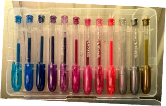
For example, in Figure 4.4, because the pens are lined up neatly in the box, the amount of ink remaining in each pen produces a graph of ‘amount of ink’ against ‘pen’. You can sometimes see similar ‘graphs’ when looking at a row of glass jars in a kitchen cupboard.
Graphs in which the horizontal axis depicts time can be a simple way to begin.
Let’s imagine a graph of the temperature in a garden, taken at midday each day for \(10\) consecutive days (Figure 4.5).

Since there is only one temperature reading per day, there are just \(10\) data points, and there are no in-between values. It is very common in real-life situations for the domain of a function to be a set of discrete values, rather than a continuous interval.
A lot of people really struggle with the idea of a Cartesian graph, and find it difficult to see what it is showing, and it can be very helpful to build it up piece by piece.
We can think of a graph such as the one in Figure 4.5 as coming from two separate number lines - one for the time variable (the day numbers), and the other for the temperature variable (Figure 4.6).

The number line for ‘Day’ shows the domain of the function, which is the \(10\) days on which a temperature was recorded. The number line for ‘Temperature’ shows the temperatures that were recorded on those days in degrees Celsuis.
However, these two separate number lines cannot show the function that relates these two sets of values. The important thing about the function is that the points on these two number lines are linked together. So, to show this we need to keep track of which temperature is associated with which day, and one way to do this is by joining the corresponding points with lines (Figure 4.7).

If we look carefully, we can see that, in this case, the temperature values are a function of the day values, but not vice versa. Given any day, the function tells us what temperature it was in the garden on that day. But given a temperature, there could be more than one day corresponding to that temperature.
It turns out that Day \(4\) and Day \(9\) both happened to have the same temperature. You might have noticed in Figure 4.6 that while there were \(10\) dots on the Day number line, there were only \(9\) dots on the Temperature number line. That is because two of the days had the same temperature. So there is no function from temperature to day.
Two days might have one temperature, but one day cannot have two temperatures at the same time (at midday) in the same place (this garden). So, time is not a function of temperature. For this reason, we might want to put arrows from day to temperature on the double number line diagram (Figure 4.8).

The genius of René Descartes was to realise that all of this would be much more convenient if we rotated the Temperature axis through \(90{^\circ}\), keeping the links between the Day and the Temperature (Figure 4.9).

And that this would be even clearer if we placed the points off the axes at the corresponding positions shown in Figure 4.10.

To the teacher, this lengthy process may seem unnecessary. But many learners do not really follow what graphs are showing. I think walking learners through this development of the modern Cartesian representation can help with understanding where it comes from and what it means. Every learner should see this once.
4.3.2 Discrete and continuous variables
It is sometimes helpful to ‘join the dots’ in discrete data to help highlight the pattern and make dots that are further out easier to spot (Figure 4.11).

But it isn’t at all plausible that the temperature actually follows this jerky dot-to-dot profile in between the actual measurements. If, instead of taking one reading per day, we were to set up continuous temperature monitoring in the garden, we would expect to get a nice smooth output, something like that shown in Figure 4.12. Here, we are thinking of temperature as a continuous function of time.

Functions can also be continuous, but with pieces missing from the domain. For example, we could imagine the temperature probe losing its internet connection some time after midday on Day \(5\), and reacquiring the connection later, which could lead to a graph such as the one shown in Figure 4.13.

4.3.3 Restricting the domain
However, not every squiggle you can draw on graph is a function.
The curve shown in Figure 4.14 is not a function, because some times seem to have multiple temperatures, which is impossible. No sequence of temperature measurements over time could lead to a graph looking like this.

Such a curve fails the vertical line test, which is way of checking that something is a function by sliding a vertical line along the horizontal axis. The vertical line must find a unique value on the curve for every different horizontal position. This relationship fails for vertical lines such as the ones shown in Figure 4.15.

However, we can make this into a function if we just remove the awkward parts from the domain (Figure 4.16). Every value in the (now restricted) domain has exactly one value of temperature. Restricting the domain is a very useful way of making functions out of non-functions.

4.4 Inverse functions
A really important theme throughout mathematics is the idea of an inverse. Whenever we transform something in some way, we always want to know whether we could go back, and reverse the process.
We considered this in Chapter 1 in the context of ‘undoing’ an addition or a multiplication by using a subtraction or a division. Subtracting \(7\) is the inverse of adding \(7\), and adding \(7\) is the inverse of subtracting \(7\). Dividing by \(7\) is the inverse of multiplying by \(7\), and multiplying by \(7\) is the inverse of dividing by \(7\).
In function notation, we could say that if \(f(x) = x + 7\), then \(f^{- 1}(x) = x - 7\), and if \(g(x) = 7x\), then \(g^{- 1}(x) = \dfrac{x}{7}\).
Although \(f^{- 1}\) doesn’t mean ‘\(f\) to the power of negative \(1\)’ and isn’t equal to \(\dfrac{1}{f}\), the notation does make sense, because, for example, \(7^{- 1}\) is the multiplicative inverse (reciprocal) of \(7\), since \(7 \times 7^{- 1} = 1\), so we could write that if \(g(x) = 7x\), then \(g^{- 1}(x) = 7^{- 1}x\).
Since an inverse function has to be a function, a function can only have an inverse if it is one-to-one, meaning that every input has a different output. If the outputs from two inputs were equal, then that function couldn’t have an inverse, because if we were to put one of those outputs into the inverse function, there would be two possible answers, and that isn’t allowed for a function.
We can test to see if a function is one-to-one by doing a horizontal line test. If a horizontal line crosses the curve more than once, it means that one output corresponds to more than one input, so we can’t invert the function.
We saw this with the temperature-in-the-garden example in Section 4.3.1. Day \(4\) and Day \(9\) both had the same temperature. This didn’t stop the relationship from Day to Temperature from being a function, because every day had a single, unique temperature. But it meant that there was no inverse function, because one of the temperatures could have come from either of those two days.
To get an inverse, we would have to remove either Day \(4\) or Day \(9\) from the domain of the original function. This would make the original function one-to-one, meaning that each temperature would now have one and only one day. A one-to-one function is invertible (i.e. has an inverse).
For example, the function \(y = x^{2}\) has no inverse, because inputs like \(3\) and \(-3\) both go to \(9\), and so, in the inverse function, we wouldn’t know what the output should be for an input of \(9\) (would it be \(3\) or would it be \(-3\)?).
However, if we throw away half of the \(y = x^{2}\) function, by making it the function ‘\(y = x^{2}\) when \(x \geq 0\)’, say, then this problem goes away. Now, the only way to get \(9\) from this function is to input \(3\) (because \(-3\) is no longer in the domain), and therefore the inverse function \(y = \sqrt{x}\) can take in \(9\) and give out the single answer of \(3\).
Here, we are restricting the domain, not to make something into a function (\(y = x^{2}\) was already a function), but to make it into a one-to-one function. This is why the domain is an essential part of any function. The two functions described below look similar, but are completely different functions.

In solving an equation like \(x^{2} = 9\), we get \(x = \pm \sqrt{9} = \pm 3\).
We take \(\sqrt{9}\) to mean \(3\), and not ‘\(3\) or \(-3\)’, because we want \(y = \sqrt{x}\) to be a single-valued function.
If we wanted to indicate both square roots of \(x\), i.e., \(\sqrt{x}\) and \(- \sqrt{x}\), like we do in the quadratic formula (Chapter 2), then we would have to write \(\pm \sqrt{x}\). But \(y = \pm \sqrt{x}\) is not a function, because \(\pm \sqrt{9}\) has two values, \(3\) and \(-3\) (Figure 4.17).

Learners are often confused about this, but \(\sqrt{9}\) is a number, whereas \(\pm \sqrt{9}\) is not a number (because it is two numbers).
This means that when simplifying surds (Chapter 2), we can write, for example, \(\sqrt{12} = \sqrt{4}\sqrt{3} = 2\sqrt{3}\), without needing to include any \(\pm\) symbols. However, when someone says in words ‘the square root of \(9\)’, it may be unclear whether they mean ‘the positive square root of \(9\)’ or ‘both square roots of \(9\)’.
A memorable task is for learners to use graph-drawing software to sketch the graphs of some functions involving the \(\pm\) symbol.3
4.5 Displacement-time and velocity-time graphs
A good way to help learners develop their understanding of what graphs are showing is to think about displacement-time or velocity-time graphs of everyday processes, such as the subsequent motion of a ball after it is thrown vertically up into the air. If you ask learners to sketch how they think these graphs will look, they may produce quite a wide variety of different ideas, which can make for an interesting discussion.
The vertical displacement of the ball upwards will increase with time up to a maximum value, and then decrease, so an inverted-U-shaped parabola will be produced for the first part of the displacement-time graph.
When the ball hits the ground, it will repeat the same shape of curve, but due to energy losses caused by resistive forces (e.g. air resistance, viscous damping inside the ball, since its collision with the ground won’t be perfectly elastic), it will attain lower and lower heights with each successive bounce, meaning that the graph will look something like the one shown in Figure 4.18(a).

The corresponding velocity-time graph will look quite different.
It will consist of straight line segments, because in a uniform gravitational field the velocity will change at a constant rate (equal to the acceleration due to gravity).
The velocity of the ball will decrease steadily until it reaches zero, when the ball attains its maximum height. The velocity will then become negative as the ball descends. When the ball hits the ground, if it bounces, its velocity will very quickly change from negative to positive. Because it loses some energy when it hits the ground, the magnitude of its new velocity will be less, but the slope of the line will be the same, because the acceleration due to gravity is constant. This means that the ball will spend less time in the air before each successive bounce, shown by the dashed vertical lines getting closer together over time (Figure 4.18(b)).
Learners may not have the scientific knowledge to know all these details, but they should be able to interpret the graphs and make sense of how they look in terms of what they do know about the real world.
4.6 Functions of more than one variable
Functions of more than one variable may sound like an advanced topic that learners would only meet when much older and studying topics such as partial differentiation, but it isn’t really. Everyone knows that in everyday life in many situations an outcome depends on the values of more than one variable. It happens all the time in school-level science, where formulae frequently have more than two different letters in them. For example, the volume of a gas depends on both its pressure and its temperature, so volume is a function of (at least) two variables (pressure and temperature).
It also happens often in applications in school mathematics. The distance travelled by a car depends on its mean speed and the time it has been travelling, so distance is a function of these two variables.
It is also common in pure mathematics.
For example, the area of a parallelogram is equal to the base \(b\) multiplied by the height \(h\), so the area is a function of two variables, \(b\) and \(h\) (Chapter 3).
We could write \(A(b,h) = bh\) if we wanted to. To draw a graph of this function would require three dimensions (Figure 4.19). The domain of both \(b\) and \(h\) are restricted to be positive, since lengths have to be greater than zero.

Another example would be the size of the third angle of a triangle as a function of the sizes of the other two angles (Chapter 3).
If we call the angles in degrees \(A\), \(B\) and \(C\), we could write \(A(B,C) = 180{^\circ} - B - C\) (Figure 4.20).

And if we rearrange the formula \(a^{2} + b^{2} = c^{2}\) for Pythagoras’ Theorem (Chapter 3) to find the length of the hypotenuse \(c\), as \(c = \sqrt{a^{2} + b^{2}}\), we can think of \(c\) as being a function of both \(a\) and \(b\) (Figure 4.21).

All of these examples are perfectly good functions – they just happen to have more than one independent variable.
When learners are rearranging equations to make a different letter the subject, such as when transforming \(A = bh\) into \(h = \dfrac{A}{b}\), they sometimes wonder if they are ‘finding the inverse’. Converting \(A = 3h\) into \(h = \dfrac{A}{3}\) would be finding the inverse of the function \(A(h) = 3h\), and it feels very similar, so it is helpful to realise that \(A = bh\) is also a function, but of two variables.
Graph-drawing software is essential here, if you want to show these.
4.7 Graphs that are not functions
Not all the graphs that learners meet in school are functions.
They may think that statistical graphs are not functions, because there is ‘no formula’, but we have seen that having a formula isn’t necessary for something to be a function. What matters is that each input has exactly one output (no more, no fewer).
4.7.1 Vertical lines and circles
The most common examples of non-function graphs in pure mathematics in school are vertical lines and circles (Figure 4.22). These aren’t functions, because they fail the vertical line test.

4.7.2 Scatter graphs
Although scientific/statistical graphs such as the temperature in the garden are functions, one statistical graph that is rarely a function is a scatter graph (scatter plot). In a scatter graph, the same \(x\) value can have more than one \(y\) value associated with it. This becomes increasingly likely as the sample size increases.
For example, suppose we gather a random sample of people from some population, and for each person measure both their height and the width of their handspan. To within whatever level of accuracy we are working, it is quite plausible that we could find two people with the same hand span. Are they guaranteed to have the same height? If there is a correlation between hand span and height, then we would expect the heights of those two people to be similar. Nevertheless, we have no right to expect that they will be exactly equal.
This means that if we plot height on the vertical axis and hand span on the horizontal axis, we could draw a vertical line through the hand span width corresponding to our two people, and it would hit two different points directly above it, one for each of their heights (Figure 4.23). This double-value output prevents the relationship from being a function.

A nice way to introduce scatter graphs is to use people (or objects) as the points, and have them stand (or place the objects) at the appropriate positions on a large pair of axes laid out on a flat surface. A collection of small objects could be provided, and then learners could suggest a list of possible variables (e.g. mass, height, cost, colour, width, etc.), and then choose two of these to use to make a graph.
An interesting example is to use drinking glasses or cups and let the two variables be the height and the circumference of the rim. Learners can first try to order the vessels by height, which is quite easy, and then by rim circumference, which is much harder. Then, they can estimate where to place each vessel on the two-dimensional graph (Figure 4.24). Finally, they can make some measurements to check, using a tape measure.

They may be surprised that almost all glasses have a greater circumference than height, even a champagne glass. It has been said that the only common object you can drink from that has a greater height than circumference is a straw!
As we have seen, functions are extremely useful, but with scatter graphs we don’t want to restrict the domain to find a function – that would mean excluding data for no good reason, and would bias our conclusions. But if we want to summarise our data and make predictions, we might want to find a function that tells us on average what height we would predict for a given handspan, even a handspan that doesn’t precisely match any of the values in our sample.
This is what a regression line gives us (Figure 4.25), and these are often called lines of best fit or trend lines in school mathematics.

We want to find a straight-line function that gets as close as it can to all the data points in our sample. There are different ways of trying to do this, so there isn’t really one ‘line of best fit’ that is ‘the right answer’. In fact, finding a regression line for predicting height from handspan is a different question from finding a regression line for predicting handspan from height, because you either want to model the variation in the heights or the variation in the handspans.4
It often worries learners that a line of best fit may not pass exactly through any of the data points, and so they feel it is somehow ‘wrong’. But that misunderstands what we are trying to do. The model is an attempt to capture the overall pattern of the data, and give a single prediction of height (i.e. a function) for every different handspan we might want to know about. We are not trying to fit each individual data point but the overall pattern across all of them.
Making predictions in between data points (interpolation) is likely to be more accurate than making predictions for values far away from any of the data points (extrapolation). Once we depart from the hand span range of the majority of the data you have collected, any predictions your model makes are likely to be much less reliable, and may eventually become quite absurd.
For example, the equation of our regression line, with \(x\) as the handspan in cm and \(y\) as the height in cm, turns out to be \(y = 1.17x + 150.7\). This means that the intercept is \(150.7\) cm, which would be the prediction of the height of someone with zero handspan! We could even predict height values for negative handspans, but clearly this doesn’t correspond to anything sensible in the real world. The model is based on data within a certain range, where it may be useful, but all models break down eventually, and depart so far from reality that they become no longer of any practical use (see Chapter 5).
4.8 Straight lines that go through the origin
Straight lines are the most important functions in mathematics. They crop up all the time. Even graphs which aren’t straight can often be approximated by straight lines, and often the approximation will be good enough for whatever our purpose is. When learners study differentiation in calculus (Section 4.11.10.1), they may think of this as the study of ‘local straightness’, meaning curves which look straight if you zoom in far enough (see Section 4.11.10.1). Straight lines are so convenient to handle, because everything we know about thinking multiplicatively applies.
We saw in Chapter 1 that to think multiplicatively we need linear relationships with true zeroes (Section 4.2.2). We always included zero on the number lines in Chapter 1, because, when multiplying, every number has meaning only in relation to zero. Multiplication by \(m\) moves the number \(m\) times as far away from zero as it was before.
All our multiplicative relationships fit the equation \(y = mx\), where \(m\) is the multiplier. When drawing a graph of a \(y = mx\) relationship, we get a straight line through the origin, such as \(y = 3x\), shown in Figure 4.26.

By a certain age, learners may have got used to this form of the graph, but not really have much sense of why it has to be a straight line. Why couldn’t it be a curve instead?
The point about multiplicative relationships that we saw in Chapter 1 is that they have a constant multiplier, that doesn’t change. This is the \(m\) in \(y = mx\). When we increment \(x\) by any amount \(\mathrm{\Delta}\), \(y\) increases by \(m\) times as much.
Formally, we could write
\[m(x + \mathrm{\Delta}) = mx + m\mathrm{\Delta} = y + m\mathrm{\Delta}.\]
The \(\mathrm{\Delta}\) symbols in this make it look more ‘advanced’ than it needs to; it is just adding and multiplying. We could always replace \(\mathrm{\Delta}\) with any number, like \(5\), if we prefer:
\[m(x + 5) = mx + 5m = y + 5m.\]
The point is that when \(x\) increases, by any amount, say \(5\), then \(y\) increases by \(m\) times as much as that amount. But since \(m\) is a constant, \(5m\) will also be a constant.
Similar triangles ensure that the gradient remains \(m\), and because the gradient (or multiplier) is constant, we get a straight line.
For curves, such as a parabola, say (see Section 4.10.2), this wouldn’t work, because, for example, \[m(x + 5)^{2} \neq mx^{2} + 5^{2}m.\]
4.9 Straight lines that don’t go through the origin
I would not move on to this until learners are extremely confident with Section 4.8 and Chapter 1.
4.9.1 Transforming into \(\boldsymbol{y' = mx}\)
When a straight line doesn’t go through the origin, that just tells us we are using the ‘wrong’ zero! If we had chosen the ‘right’ zero for our \(y\) variable, it would have been the familiar \(y = mx\) line.
I recommend spending a lot of time on \(y = mx\) in the context of thinking multiplicatively before adding the complication of the ’\(+ c’\).
I think it is usually easier to understand \(y = mx + c\) by transforming it into \(y - c = mx\). By modifying the \(y\) variable from \(y\) to \(y’ = y - c\), we slide all the points a distance \(c\) vertically down, giving a straight-line-through-the-origin relationship, just with a different output variable: \(y’ = mx\).5
Once you have done that, all the thinking multiplicatively that learners are familiar with applies exactly as before, just with the \(y’\) variable, rather than the \(y\). This may look complicated in algebra, but geometrically it is just translating the graph to its ‘natural’ position, where the line goes nicely through the origin.
For example, in many simple models, there is a ‘fixed cost’ and a ‘rate’. We could have a scenario of hiring a bike, where there might be a fixed cost of \(£5\), plus an additional, timed cost of \(£10\) per hour that the bike is used.
A graph of the total cost \(£y\) against \(x\), the number of hours used, will be a straight line with gradient \(10\) and intercept \(5\) (Figure 4.27(a)), so \(y = 10x + 5\).

However, if we focus on the timed cost, which is the variable part, then this is directly proportional to the time taken, and so gives a straight line through the origin (Figure 4.27(b)). The timed cost \(£y'\) is just \(10\) times \(x\), the number of hours, so \(y' = 10x\).
To get the total cost \(£y\) from this, we just need to add on the fixed charge, \(£5\), which doesn’t depend on the time.
So, \[y = y' + 5 = 10x + 5.\]
Up to here, we have defined \(x\) a bit casually as ‘the number of hours the bike is used’, assuming that we are rounding this number up to the next hour, so for example \(2\frac{1}{4}\) hours would be costed as \(3\) hours. This assumes that the hourly charge is made for every hour or part hour that the bike is kept.
If this is how the charging works, we could define \(x\) as being the number of hours or part hours for which the boat is used. Then, \(x\) is a discrete variable that has to be a positive integer. However, if we want \(x\) to be the actual amount of time (in hours) that the bike was used, then our graphs need to be a little different, as we will now see.
A pure mathematics task to develop thinking about straight lines that don’t go through the origin involves finding as many equations as possible for lines that all pass through a common point, such as \((2,\ 3)\).6
4.9.2 The floor and ceiling functions
Two extremely useful ‘straight line’ functions for modelling are the floor and the ceiling functions.
The floor function \(y = \left\lfloor x \right\rfloor\) is the greatest integer less than or equal to \(x\), and the ceiling function \(y = \left\lceil x \right\rceil\) is the least integer greater than or equal to \(x\).
Saying it like this makes them sound very complicated, but they are actually quite familiar ideas from everyday situations, as we will see. Both of these functions are piecewise (i.e. glued together) combinations of flat, constant functions \(y = c\) (i.e. with \(m = 0\)).7
Using the ceiling function (i.e. rounding up non-integers to the next integer), our graph would look as in Figure 4.28, where every time \(x\) between, say, \(2\) hours and \(3\) hours is charged as \(3\) hours.

The floor function is much more familiar to learners, because it is how age is rounded. When someone is \(11.8\) years old, they are \(11\), not \(12\), even though they have been alive for nearly \(12\) years. There are some quite challenging puzzles that we can pose related to this aspect of age:8
Abdul is \(10\) and Bella is \(12\).
How old will Bella be when Abdul is \(12\)?
Why is the answer not as obvious as it might seem?
4.9.3 Alternative forms of a straight line
There is actually more than one way to write the equation of a straight line; to simply say that a straight line is \(y = mx + c\) is too simplistic.9
We have already seen that it may be helpful to write \(y = mx + c\) as \(y - c = mx\), but there are further possible variations.
For example, all six equations below represent the same line - although you might quibble that the second one is the line with the point \(( - 1,\ - 12)\) missing, since \(\dfrac{0}{0}\) is undefined.
\[ \begin{array}{|c|c|c|} \hline \rule[-4.5ex]{0pt}{10ex} \text{ \hspace{1.6cm} } y = 3x - 9 \text{ \hspace{1.6cm} } & \text{ \hspace{1.3cm} } \displaystyle \frac{y + 12}{x + 1} = 3 \text{ \hspace{1.3cm} } & \text{ \hspace{1.2cm} } y + 12 = 3(x + 1) \text{ \hspace{1.2cm} } \\ \hline \rule[-4.5ex]{0pt}{10ex} 3x - y - 9 = 0 & \mathbf{r} = \begin{pmatrix} -1 \\ -12 \end{pmatrix} + \lambda\begin{pmatrix} 1 \\ 3 \end{pmatrix} & \displaystyle \frac{x}{3} + \frac{y}{(- 9)} = 1 \\ \hline \end{array} \]
I once saw a mathematics lesson in which the teacher drew a \(45^\circ\) line through the origin and asked the class what the equation of the line was. One learner said “\(x = y\)”, and the teacher said, “Yes, but we write it as \(y = x\). We always put the \(y\) first.” And I wondered about this response – do “we”?
The equation \(x = y\) is exactly equivalent to \(y = x\); they are exactly the same equation, just written the opposite way round. Teachers often stress that the equals sign is symmetrical, so that giving the solution to an equation as \(5 = x\), say, is exactly equivalent to giving it as \(x = 5\).10
However, there can be some benefits to putting the \(y\) first when it comes to equations of straight lines, and seeing \(x\) as the ‘independent variable’. In this way of thinking, as we have seen, \(y = 5\) is a function, whereas \(x = 5\) isn’t, even though \(x = 5\) represents a perfectly good line in the \(xy\) plane.
The table below shows six different forms of the equation of a line, along with some possible pros and cons.

The gradient-intercept form \(y = mx + c\) (#1) dominates in school mathematics, to the extent that many learners will see this as ‘the’ equation of a line. This fits with a ‘functions’ interpretation, and is useful when we want the gradient to be explicit, such as when it corresponds to a rate of something tangible in a real-life situation, such as the cost per hour of hiring a bike, or when we want to visualise the slope of the graph.
One limitation of #1 is that it does not encompass vertical lines. I have sometimes heard teachers say, “If it can’t be rearranged into the form \(y = mx + c\), then it isn’t a straight line”. But, while this is true for functions of \(x\), it is not strictly correct, because vertical lines take the form \(x = k\), which is not rearrangeable into the form \(y = mx + c\).
This problem is particularly apparent when students are first introduced to the equation of a line, because usually the first examples they meet are vertical and horizontal lines.
Lines like \(y = 3\) are easy to plot, because “the \(y\)-coordinate is \(3\) all the way along, so \(y\) is always equal to \(3\)”, and similarly for vertical lines, like \(x = 2\).
But while the \(y=c\) fit nicely into the \(y = mx + c\) form (with \(m = 0\), because the gradient is zero), the \(x=k\) ones do not, because lines of the form \(x = k\) have ‘infinite’ gradient, and are not functions of \(x\). So, we have to be careful not to say that every straight line fits \(y = mx + c\) and is a function, because vertical lines don’t and aren’t.
In contrast to this, all lines in the \(xy\) plane can be represented in the form \(ax + by = c\ \)(form #4 in the table above); lines parallel to the \(x\)-axis by taking \(a = 0\), and lines parallel to the \(y\)-axis by taking \(b = 0\). This form does not treat \(y\) as a function of \(x\); instead, it treats the variables \(x\) and \(y\) symmetrically, and is particularly useful when graph sketching in the context of linear-programming problems, where inequalities like \(3x + 4y < 12\) need to be shaded (see Section 4.11.5).
Sometimes, learners’ first instinct with these is to rearrange an equation like \(3x + 4y = 12\) into \(y = - \frac{3}{4}x + 3\), find the \(y\)-intercept \((0,\ 3)\), and then attempt to draw a line going ‘\(1\) along and \(\frac{3}{4}\) down’. This is fiddly and the line is probably unlikely to pass exactly through \((4,\ 0)\) on the \(x\)-axis by the time it gets there!
Alternatively, by leaving the equation in the form \(ax + by = c\), it is much easier to substitute the values \(x = 0\) and \(y = 0\) to find both intercepts and join them together - perhaps checking a third convenient integer point, just to make sure. The form \(y = mx + c\) privileges the \(y\)-intercept as particularly special - indeed, often it is simply called “the intercept” - whereas with \(ax + by = c\) it is equally easy to find either the \(x\)- or the \(y\)-intercepts.
Older learners are often expected to ‘move on’ from the familiarity of #1 and begin to work with lines expressed as \(\dfrac{y - y_{1}}{x - x_{1}} = m\) (#2 in the table above).
Here, \((x,\ y)\) is a general point on the line and \((x_{1},y_{1})\) is a particular fixed, given point on the line, and this distinction is often difficult for learners, since they symbolically look so similar.
It is also problematic that \((x_{1},y_{1})\) does not actually satisfy the equation that is created, since it leads to \(\frac{0}{0}\), even though it is the one point we are absolutely sure does lie on the line!
The form \(y - y_{1} = m(x - x_{1})\) (#3 in the table above) avoids this problem, and is a good example of where deliberately not simplifying something can make the structure more transparent, because in \(y - y_{1} = m(x - x_{1})\) we can “see” the m and the \((x_{1},y_{1})\) explicitly. Simplification, of course, is all that distinguishes #2 and #3 from #1.
Finally in the table above, #6 is perhaps handy if you want to write down the equation of a line given the two intercepts.
For example, a line passing through \((5,\ 0)\) and \((0,\ 8)\) can be written by simply placing the numbers \(5\) and \(8\) in the denominators, as: \[\frac{x}{5} + \frac{y}{8} = 1.\]
For me, this use case is a bit too niche to make this form of much general importance.
While we do of course have to teach \(y = mx + c\) (#1), and with older learners we may also need to teach vector equations of a line (#5), I think there is scope for plenty of use of #3 and #4 at all stages.
4.10 Curves
There are infinitely many weird and wonderful curves that learners can plot using graph-drawing software, and which may be useful functions. The table below shows one informal way to categorise functions that appear in school, so we perceive a fixed number of important different kinds, rather than just an endless variety.

We will consider each of these in turn in the sections below.
4.10.1 Trigonometric functions
Sinusoidal functions (sine and cosine) jiggle up and down forever (Figure 4.29). They are useful for modelling oscillating phenomena, like electromagnetic waves or tides.

You can create sine waves in the classroom by having one learner walk around a circle while two others track the first one’s position along two perpendicular axes. One of the trackers will end up following sine and the other cosine (Figure 4.30). This parallels how these trigonometric functions were introduced in Chapter 3.

The tangent function is also periodic, but with a period of \(180{^\circ}\), rather than \(360{^\circ},\) and contains vertical asymptotes (see Section 4.10.5).
4.10.2 Polynomial functions
These contain terms that have positive integer powers of \(x\) and a constant only. They go up and down for a while and then ‘run out of jiggle’.
Figure 4.31 shows the graph of \(y = x^{5} - 5x^{3} + 4x + 1\).

It has four turning points (places where the direction changes) and five zeroes (places where \(y = 0\)) – the maximum number of each that a \(5\)th-order polynomial can have.
By far the most prominent of the polynomial curves in school mathematics are the quadratics. They come as ‘happy’ and ‘sad’ parabolas (Figure 4.32).

‘Happy’ ones (with a positive coefficient of \(x^{2}\)) have a minimum point and ‘sad’ ones (with a negative coefficient of \(x^{2}\)) have a maximum point. With just one stationary point, a minimum has to be a global minimum, and maximum has to be a global maximum. But for the quintic shown in Figure 4.31, both maxima are exceeded by the \(y\) values at other points, and neither minimum is the lowest value the function takes anywhere, so we call these local maxima and minima, rather than global ones.
Because of their shapes, quadratics are great for modelling U-shaped and inverted-U-shaped phenomena, such as things that increase up to a point but then decrease. An example of an inverted-U-shaped curve could be the profit you might make from selling something as you increase its price. To start with, people pay the higher price, and you make more money, but once the price gets too high people don’t buy as much of it, or switch to a competitor, and then your profits go down. An inverted U-shaped graph like this could be modelled by a quadratic equation. (Marginal cost curves and total revenue curves are often U-shaped and inverted-U-shaped respectively.)
The other common use of inverted-U parabolas is to model projectile motion, because ‘what goes up, must come down’ (see Section 4.5).
Because quadratic functions have a single turning point, they can cross the \(x\) axis a maximum of twice. Unless they are horizontal, straight lines always have to cross the \(x\) axis once, but quadratics can cross the \(x\) axis twice, just touch the \(x\) axis at one point, or miss the \(x\) axis altogether, as shown in Figure 4.33.

The values of \(x\) for which the curve intersects the \(x\) axis are called the zeroes of the function, or the roots of the equation in which \(y\) is set equal to zero. Finding these values corresponds to solving a quadratic equation (Chapter 2).
4.10.3 Exponential functions
We have seen that sinusoidal functions go up and down forever, and polynomials go up and down for a while, and then run out of jiggle.
Exponentials just go up and up (exponential growth) or down and down (exponential decay) (Figure 4.34)!

Exponential functions are very useful for modelling situations in which ‘the more you have, the more you get’ – positive feedback loops – such as when bacteria are growing with plenty to feed on. The more bacteria you have at any point, the more new ones you are going to get. The rate of growth is not just a steady positive constant; it is proportional to how many bacteria there are at that point, and so the steepness of the curve increases, and does so at an increasing rate.
The shape of an exponential growth curve is nothing like the shape of a 'happy’ parabola. The rate of increase in slope of a parabola is constant. It gets steeper and steeper, but at a constant rate. An exponential curve gets steeper and steeper but at an increasing rate.
When people say that something ‘increases exponentially’, they often just mean that it increases ‘a lot’. For example, suppose not many people came to the cinema yesterday, and today it is crowded. Then someone might say there has been an ‘exponential increase’ in the number of people. But that isn’t a mathematically precise statement. Really, for something to increase exponentially, all we mean is that the rate of growth is proportional to how much there currently is.
Exponential growth can be shallow but still be exponential, such as for the negative values of \(x\) in Figure 4.34(a).
On an exponential curve, the slope of the curve at any point is proportional to the height of the curve at that point.
For example, on the curve \(y = 3^{x}\), when we move \(1\) unit to the right, \(y\) becomes \(3\) times as much, and the slope also becomes \(3\) times as much, as shown in Figure 4.35.

Exponential decay is equally important. In this case, \(y\) decreases at a rate proportional to how much \(y\) there currently is.
The temperature of a cooling cup of tea is a good example. The tea is heading downwards in temperature, towards being at the same temperature as its surroundings. But it doesn’t head there in a straight line and then suddenly level off when it hits room temperature, as in Figure 4.36.

Instead, the tea loses heat faster at the start, when it is much hotter than its surroundings.
A good model is to assume that the rate at which it loses heat is proportional to the difference between its temperature and the temperature of its surroundings (Newton’s Law of Cooling). This gives us an exponential decrease in temperature (Figure 4.37).

In theory (i.e. according to our mathematical model), the gap between the temperature of the tea and the temperature of the room decreases continuously, but never quite becomes zero. We can find a difference as small as we wish between the tea temperature and the room temperature, just by going out far enough to the right on the graph. Unless we could go infinitely far to the right (i.e. wait forever), we would never find the difference to be precisely equal to zero.
Of course, in reality the temperature of the tea will eventually be indistinguishable from room temperature, but our model isn’t refined enough to tell us exactly when this will happen. All models are just convenient and useful approximations to reality – never the absolute truth.
Exponential decay has many applications in electronic circuits and radioactive decay and generally when something is ‘dying away’.
The name exponent means the same as index, and refers to the \(x\) being the index of some base, such as \(3\) in \(y = 3^{\pm x}\).
The larger the base number, the faster the growth or decay. If the base were \(1\), then \(y = 1^{x} = 1\), and we would have a flat, constant function. However, even if the base is just ever so slightly greater than \(1\), we get growth that, if you wait long enough, becomes considerable.
For example, consider the function \(y = {1.1}^{x}\).
This function describes a \(10\%\) increase for every increase in \(x\) of \(1\) unit. This could be a model for a \(10\%\) per year compound interest rate.
This will double your money when \[{1.1}^{x} = 2,\] which is when \(x = 7.27\) (we can find this by trial and improvement, or by using logarithms), meaning that, if nothing else changes, after \(8\) years you will have more than twice the amount you began with.
The function \(y = {0.8}^{x}\) corresponds to a \(20\%\) decrease for every increase in \(x\) of \(1\) unit.
This could model the depreciation of an item that becomes \(20\%\) less valuable every year. After \(11\) years, it will be worth less than \(10\%\) of its original value, because \({0.8}^{11} = 0.09\), correct to \(2\) decimal places, which is less than \(0.1\).
We can write the function \(y = {0.8}^{x}\) equivalently as \(y = {1.25}^{- x}\), with a base greater than \(1\) and a negative exponent. (The numbers \(0.8\) and \(1.25\) are reciprocals of each other, since their product is \(1\).) These are two equivalent ways of writing the same exponential function, which often confuses learners.
The special base of \(e = 2.71828\ldots\) has the very useful feature that the rate of growth is not just proportional to \(y\) but exactly equal to it (i.e. the constant of proportionality is \(1\)). The function \(y = e^{x}\) has many important applications in science and mathematics.
Exponential growth is also called geometric growth, and geometric series/progressions are the same thing as exponential series/progressions (see Section 4.11.3.1).
4.10.4 Reciprocal graphs
The final main category of functions that learners need to encounter are reciprocal functions, such as \(y = \dfrac{1}{x}\).
Some interesting features of \(y = \dfrac{1}{x}\ \)are that it has a vertical asymptote at \(x = 0\), a horizontal asymptote at \(y = 0\), and the curve is discontinuous, meaning (informally) that you can’t draw it without taking your pen off the paper (Figure 4.38).

The curve consists of two distinct branches either side of the vertical asymptote. It is always going downhill (from left to right) wherever you are on the curve.
4.10.5 More about asymptotes
When we considered exponential functions like \(y = 3^{\pm x}\), we noted that for these functions the \(x\) axis (\(y = 0\)) is a horizontal asymptote - a line which the curve gets arbitrarily close to, as \(x\) gets arbitrarily large.11
‘Arbitrarily close’ just means ‘as close as you like’; ‘arbitrarily large’ just means ‘as large as you like’. These can be useful terms to use when talking about the behaviour of functions.
Functions can cross their horizontal asymptotes, so it is a mistake to say that a function ‘gets closer and closer to its asymptote, but never reaches it’. For example, the function shown in Figure 4.39 has a horizontal asymptote at \(y = 0\), but crosses this at \(x = 0.4\). The asymptotic behaviour depends only on what happens when \(|x|\) gets very large. For smallish values of \(x\), anything can happen!

The other problem with the ‘closer and closer to’ language for asymptotes is that if, say, \(\dfrac{1}{x}\) gets ‘closer and closer’ to \(y = 0\), it also, necessarily, gets ‘closer and closer’ to any horizontal line below \(y = 0\), such as \(y = - 20\).
Getting ‘closer and closer’ is not what makes something an asymptote. The important feature is that, beyond a certain \(x\) value, the value \(\dfrac{1}{x}\) gets as close as you wish to zero. However close to zero you want \(\dfrac{1}{x}\) to get, it will get closer than that, and remain closer than that, beyond some suitably chosen \(x\).
For example, if you wanted \(\dfrac{1}{x}\) to be less than \(0.001\) away from zero, say, then provided you chose values of \(x\) greater than \(1000\), it would be. And you can do this, no matter how small a value for \(\dfrac{1}{x}\) you care to choose. That is the nature of what an asymptote is.
Some functions, like \(y = \dfrac{1}{x}\), have vertical asymptotes. (The function \(y = \dfrac{1}{x}\) has both.)
For example, \(y = tan\ x\) has infinitely many vertical asymptotes, coming every odd number of 90\({^\circ}\), shown with vertical dashed lines in Figure 4.40.

Vertical asymptotes happen at \(x\) values at which the \(y\) values become arbitrarily large as you get arbitrarily close to the \(x\) value.
The \(x\) value of the asymptote itself may not be in the domain of the function, because the function may not be defined for that \(x\) value. For example, \(\tan{90{^\circ}}\) would be \(\displaystyle \frac{\sin(90{^\circ})}{\cos(90{^\circ})}\), but \(\cos(90{^\circ})\) is zero, so \(\displaystyle \frac{\sin(90{^\circ})}{\cos(90{^\circ})}\) is not defined, because it would involve dividing by zero.
4.11 What does understanding functions and graphs get us?
Learning about functions and their graphs has a great benefit in being able to manipulate and work with functions right across mathematics and visualise algebraic properties by viewing their associated graphical representations. It also allows students to model interesting scenarios mathematically and explore what happens (Chapter 5). However, beyond this, I think there are many important payoffs.
4.11.1 Negative numbers
For me, one big benefit from thinking about functions and graphs is to be able to address negative numbers properly. I tend to initially treat addition and subtraction of directed (positive and negative) numbers quite separately from multiplication and division of directed numbers. Notions that ‘two minuses make a plus’ mean quite different things in the two contexts, and can easily be confused.12
Addition and subtraction of directed numbers can be addressed by moving forwards or backwards along the number line (i.e. vector journeys, see Section 4.11.9) or by considering positive and negative payments, heights, temperatures or charges (Chapter 1).13 Learners should ultimately experience all of these, in order to enrich their understanding that ‘subtracting a negative number’ is the opposite of ‘subtracting a positive number’ or ‘adding a negative number’.14 Once learners are happy that ‘subtracting a negative number’ is ‘removing a debt’, and therefore equivalent to ‘adding a positive number’, then addition and subtraction of directed numbers is just a matter of developing fluency.15
However, I think that multiplication and division of directed numbers is much more difficult, and is better tackled in the context of \(y = mx\) graphs. When thinking multiplicatively in Chapter 1, we restricted ourselves to positive \(m\), positive \(x\) and positive \(y\) (Figure 4.41). However, once we know about negative numbers, there is no reason why we should restrict ourselves to the first quadrant.

It is very natural to extend a line like \(y = 3x\) to negative values of \(x\), and thus negative values of \(y\).
For instance, it seems very reasonable to say that if
\[3 \times 5 = 15 ,\]
then
\[3 \times ( - 5) = - 15 .\]
Learners will allow that \[3 \times ( - 5) = (-5)+(-5)+(-5)=-15,\] and similarly for other negative \(x\) values.
This gives us the complete line \(y = 3x\) shown in Figure 4.42.

We do not need a rule that says ‘\(\text{positive} \times \text{negative} = \text{negative}\)’, because we can just see it from the straight-line graph. When we go to the left of zero on the \(x\) axis, we end up below zero on the \(y\) axis, and so we have a negative outcome. We can see at a glance that this is going to happen, whatever negative number (like \(- 5\)) we multiply the \(3\) by. And this is going to work just as well for non-integer values of \(x\) (Figure 4.43).

Noticing that
\[3 \times ( - 5) = ( - 5) + ( - 5) + ( - 5) = - 15\]
is important, but the ‘repeated addition’ model of multiplication does not extend easily to non-integer multipliers, whereas straight-line graphs are highly suggestive that the in-between values work in the same way.
We can also see from the graph that changing the \(3\) to any other positive value (again, not restricted to integers) is going to give some other line in the first and third quadrants, and so this relationship generalises to any positive \(m\) (Figure 4.44).

We know what a graph like \(y = 5x\) will look like, but now we have to wonder what would happen if the \(5\) itself were negative. What would a graph like \(y = - 5x\) look like?
We already know
\[3 \times ( - 5) = - 15 .\]
If we want commutativity, then it must be true that
\[( - 5) \times 3 = - 15 ,\]
so \(y = - 5x\) has to take \(x = 3\) to \(y = - 15\) (Figure 4.45).

In a similar way, \(y = - 5x\) is going to take all the positive numbers to negative numbers, because they are all going to land somewhere in the fourth quadrant. This is not a formal proof, of course, but it is very intuitive.
So, the graph in the fourth quadrant is going to look like the line shown in Figure 4.46.

This is illustrating that ‘\(\text{negative} \times \text{positive} = \text{negative}\)’, but we already know we must have that, because we have decided we are committed to commutativity.
So, our complete \(y = - 5x\) line must look like the one shown in Figure 4.47, because by symmetry we’re extending it straight through the origin, because mathematical lines go on forever in both directions.

Now we can simply read off what happens with ‘\(\text{negative} \times \text{negative}\)’, because we can see the result in the second quadrant. For example,
\[( - 5) \times ( - 3) = 15 .\]
And the pattern is not just for this specific example, but \(y = - 5x\) is going to turn all negative \(x\)’s positive. And any other \(y = mx\) with a negative \(m\) is also bound to produce \(y\) values that are positive, whenever the \(x\) values are negative.
Multiplication by a negative number switches the sign, from positive to negative, or from negative to positive.
I like this approach to multiplication of directed numbers, because there is nothing arbitrary to be told or to have to remember. We decide we want commutativity to carry over into multiplications with directed numbers, and we see that our straight-line graphs through the origin are going to continue through the origin and out the other side. And then the ‘rules’ of multiplication of directed numbers are forced on us.
Division follows simply by going backwards, from \(y\) to \(x\), as \(x =\displaystyle \frac{y}{m}\).
For example, to discover that \(\displaystyle \frac{( - 15)}{( - 5)} = 3\), we just look at the \(y = - 5x\) graph and go from \(- 15\) on the \(y\) axis along to meet the line, and up from there to positive \(3\) on the \(x\) axis (Figure 4.48). The only number which multiplies by \(-5\) to make \(-15\) is \(+3\).

All the time learners spend figuring this out, with lots of specific examples, is not only developing their understanding of multiplication and division of directed numbers; they are also practising interpreting graphs.
4.11.2 The real numbers
Another big payoff from functions and graphs is going from the integers to the rational numbers and then to the real numbers.
Thinking multiplicatively was very much focused on positive integers to begin with, and then fractions were brought in. By this point, learners are working with rational numbers, and perhaps assuming that the rationals in between the integers basically behave ‘the same way’. It is easier to be confident of this when drawing \(y = mx\) graphs, because it is intuitive that the lines are continuous and dense: there is a number in between any two other numbers.
With \(y = mx\), we can also suggest that \(m\) need not even be rational. Once learners meet Pythagoras’ Theorem (and thus surds, such as \(\sqrt{2}\), \(\sqrt{3}\), and so on), circles (and thus \(\pi\)) and volume of cubes (and thus cube roots), they become aware of irrational numbers (Chapter 2).
Graph-drawing software (with \(m\) on a slider) makes it highly plausible that non-integer (and presumably irrational) \(m\)’s fit in nicely among the rational \(m\)’s. At school level, it would be difficult and unnecessary to try to do anything more rigorous than this.
4.11.3 Powers and roots
Learners meet powers and roots quite early on, because from a young age they are likely to gain experience of doubling and halving.
4.11.3.1 Powers
Quite young children often enjoy working out several of the early powers of \(2\):
\[1,\ 2,\ 4,\ 8,\ 16,\ 32,\ 64,\ 128,\ 256,\ 512,\ 1024,\ \ldots ,\]
and these can be referred to as the zeroth, first, second, and so on powers of \(2\).
Learners will appreciate that they go up the sequence by multiplying by \(2\) and down the sequence by dividing by \(2\) (or multiplying by \(\frac{1}{2}\)). This is all good early experience of a geometric sequence (also known as an exponential sequence).
The powers of \(2\) get big extremely quickly - hence the phrase ‘exponential increase’, and the ancient ‘grains of rice/wheat on a chessboard’ question.16 And all of this is much easier to appreciate in the context of exponential graphs, where you can see the dramatic rise of the exponential function (Figure 4.49).

A question from the Cognitive Reflection Task, designed to see if people will go with their immediate, intuitive answer, or think more slowly about it, is good for probing learners’ understanding of exponential sequences: 17
In a lake, there is a patch of lily pads.
Every day, the patch doubles in size.
If it takes \(48\) days for the patch to cover the entire lake, how long would it take for the patch to cover half of the lake?
The ‘obvious but wrong’ approach to this is to divide \(48\) by \(2\) and say \(24\) days. This is thinking linearly, rather than exponentially (Figure 4.50).

If the patch is doubling in size every day, then it must, in particular, double between the \(47\)th day and the \(48\)th day, so the correct answer is \(47\) days.
This is unintuitive, partly because doubling \(48\) times is so hard to visualise. Doubling \(48\) times corresponds to an increase by a factor of \(2^{48}\), which is \(281,474,976,710,656\), and it is extremely difficult to imagine a change in lily pad area (or anything else) by such an enormous factor! In visible terms, nothing seems to be happening on the lake until around day \(40\), when there is suddenly an explosive amount of growth.
Even quite young children soon learn about the powers of \(10\). It is interesting to ask learners of various ages, “What is the biggest number you know?” They might say ‘million’ or ‘billion’ or ‘trillion’, or even words like ‘zillion’ and ‘gazillion’, which are not actual numbers. Many adults will confuse a million with a billion, so it can be very valuable to ask how large they think these numbers are, and this quickly gets into discussing how each power of \(10\) is a power of \(10\) times every other power of \(10\).18
4.11.3.2 Roots and logarithms
The natural partner to powers is logarithms, but these are typically treated as an advanced topic, and not taught until learners are quite old. I think this is a pity, because logarithms are just the inverse of exponentials, and get us from the power back to which term that power is in the power sequence.
If the \(5\)th power of \(2\) is \(2^{5} = 32\), then logarithms answer the question, “Which power of \(2\) is equal to \(32\)?”, so the logarithm of \(32\) (to base \(2\)) is \(5\), written as \(\log_{2}{32 = 5}\). Even quite young children can understand this in words, without needing to write anything down.
In school, we tend to focus on all the squares, all the cubes, and so on, of different bases (i.e., sequences of constant index or exponent), more than on the powers of particular bases (with the exception of base \(2\) and base \(10\)). Perhaps because of this, learners often muddle up things like the squares and the powers of \(2\), even though they are completely different families.
If you ask learners to give you an example of a power of \(2\), they might give you a square, such as \(5^{2}\), because it is ‘\(5\) to the power of \(2\)’, rather than an actual power of \(2\), such as \(2^{5}\). Language around this can be confusing. The number \(8\), for example, is a third power (i.e. a cube), and in particular it is the third power of \(2\). So, ‘\(2\) to the power of \(3\)’ is a ‘power of \(2\)’, not a ‘power of \(3\)’.
One way to address this is to compare a sequence of powers in which the base is constant with a sequence of powers in which the index is constant. In the table below, the powers of \(2\) are in the second column, whereas the squares are in the second row from the bottom.

These values are shown graphically in Figure 4.51, although the smaller values are completely overshadowed by the largest ones.

Because in school we tend to think more about the rows in the table above than the columns, we more often want to know which position a number has in a row (roots) than which position a number has in a column (logarithms). If we focus on, say, the fifth powers (i.e. the fifth row from the bottom), and might want to know which position in that sequence \(32\) takes, the answer will be the fifth root of \(32\), which is \(\sqrt[5]{32} = 2\), so \(32\) comes in the second position in the fifth powers, corresponding to the fact that \(2^{5} = 32.\)
In elementary mathematics, we consider that negative numbers have no even roots (e.g. \(\sqrt[6]{- 64}\) is undefined), and, at least initially, learners are expected to assume that we are interested only in the positive even roots. So, while we would say that the cube root of \(- 64\), written \(\sqrt[3]{- 64}\) is \(- 4\), because \(( - 4)^{3} = 64\), we would say that ‘the square root’ of \(64\) is just \(8\) (Figure 4.52).

Later on, we will want learners to appreciate that \(64\) has two square roots, \(\pm 8\), since both \(8^{2}\) and \(( - 8)^{2}\) are equal to \(64\). We can write the two roots as \(\pm 8\), or as \(\pm \sqrt{64}\).
Note, as we mentioned in Section 4.4, that this means that the notation \(\sqrt{\phantom{6}}\), by convention, refers only to the positive square root, which is why we need the \(\pm\) symbol if we wish to refer to both. Similarly the \(\pm\) is needed in the quadratic formula in front of the \(\sqrt{b^{2} - 4ac}\) term, in order to give us both roots (Chapter 2).
4.11.3.3 The laws of indices
It is usual to justify the fact that, for example, \(10^{2} \times 10^{3} = 10^{5}\), or, more generally, that \(b^{x} \times b^{y} = b^{x + y}\), for any base \(b\), by writing out the powers as products.19
For example,
\[10^{2} \times 10^{3} = (10 \times 10) \times (10 \times 10 \times 10) = 10 \times 10 \times 10 \times 10 \times 10 = 10^{5} .\]
This conclusion derives from the associativity property of numbers: \(a(bc) \equiv (ab)c\). When we multiply powers, we are accumulating additional multiples of the base, and each multiplication by \(b\) increases the number of \(b\)’s multiplied together by \(1\).
We can go straight from this to ascribing meaning to non-integer values of \(x\) and \(y\), by noticing that, for example, by following the same pattern,
\[10^{\frac{1}{2}} \times 10^{\frac{1}{2}} = 10^{\frac{1}{2} + \frac{1}{2}} = 10^{1} = 10 .\]
So, if \(10^{\frac{1}{2}}\) is a number at all, then its product with itself is \(10\), and so it must be the square root of \(10\).
Similarly,
\[10^{\frac{1}{3}} \times 10^{\frac{1}{3}} \times 10^{\frac{1}{3}} = 10^{\frac{1}{3} + \frac{1}{3} + \frac{1}{3}} = 10^{1} = 10 ,\]
and so \(10^{\frac{1}{3}} = \sqrt[3]{10}\), and, in general, a product of \(n\) factors of \(10^{\frac{1}{n}}\) will be equal to \(1\), and so
\[10^{\frac{1}{n}} = \sqrt[n]{10}\] and, in general, \[b^{\frac{1}{n}} = \sqrt[n]{b},\]
the \(n\)th root of \(b\).
For this to work for all values of \(n\), we need \(b \geq 0\) here, because even \(n\)th roots of negative numbers are not real (i.e. do not exist for learners who have not yet encountered imaginary numbers).
Subtracting \(1\) from the index is the inverse of adding \(1\), and so is going to step us back down the powers, and reduce the product by a factor of \(10\).
It is not hard to see from this that \[10^{x - y} = \frac{10^{x}}{10^{y}}\] and, by extension, that \[\frac{b^{x}}{b^{y}} = b^{x - y},\] for integer \(x\) and \(y\) and any non-zero base \(b\).
Base \(10\) is an ideal starting point. It is very convenient to begin by playing around with powers of \(10\) like this, because then the calculations are easy and familiar, and learners do not fill up their headspace calculating, and instead can step back and see the structure. If we can help them to see what is going on with base \(10\), they will readily accept that ‘the same thing’ is going to happen whatever the base, at least if we assume that the base is positive.
There are also convenient parallels here with our decimal number system, as discussed in Chapter 1 (Figure 4.53).

We can also see that if \(y = x\) then we have \(10^{x - y} = 10^{x - x} = 10^{0}\).
However, considered the other way, \(10^{x - x} = \dfrac{10^{x}}{10^{x}} = 1\), so \(10^{0}\) and \(1\) must be equal.
It is understandable that learners will want \(10^{0}\) to be equal to \(0\), because there is still some residual thought that ‘\(10\) to the power of zero’ is ‘\(10\) times zero’, or because there are ‘zero \(10\)s multiplied together’. But, when looked at in the context of the other powers of \(10\) (Figure 4.53), the zeroth and negative powers of \(10\) fit the only possible pattern, which is repeated division by \(10\).
To get a power of \(10\) that was equal to zero, we would need an extremely large negative index. We saw earlier in Section 4.10.3 that the graph of \(y = 10^{x}\) has a horizontal asymptote at \(y = 0\), as \(x \rightarrow - \infty\).
Learners sometimes think it is obvious that \(b^{xy}\) must be equal to \(\left( b^{x} \right)^{y}\), and think that this simply follows from priority of operations conventions. But I think it is not obvious that this is true.
By considering examples such as \(\left( b^{x} \right)^{3}\), which must be \(b^{x}b^{x}b^{x}\), which is equal to \(b^{x + x + x} = b^{3x}\), learners may be willing to accept that \(\left( b^{x} \right)^{y} = b^{xy}\) when \(y\) is a positive integer.
Notice that this means we have eight equivalent ways of writing a power such as \(b^{15}\), in addition to \(b^{15}\) itself:
\[\left( b^{5} \right)^{3} = b^{5}b^{5}b^{5} = b^{5 + 5 + 5} = b^{3 \times 5} = b^{5 \times 3} = b^{3 + 3 + 3 + 3 + 3} = b^{3}b^{3}b^{3}b^{3}b^{3} = \left( b^{3} \right)^{5} .\]
If we had chosen an index with more factors, as with \(b^{12}\), say, then there would be even more, because we could have started with either \(\left( b^{4} \right)^{3}\) or \(\left( b^{6} \right)^{2}.\)
By extension of this, at school level we just assume that it is all right to take it that \(\left( b^{x} \right)^{y} = b^{xy} = \left( b^{y} \right)^{x}\) for all \(x\) and \(y\).
Frequently, learners will complete tasks like ‘Simplify \(b^{3} \times b^{5}\)’ by just remembering ‘When you multiply powers, and the bases are the same, you add the indices’. This is something which is much easier to ‘just do’ than to ‘do with understanding’.20 Spending time working on the meaning not only enables learners to see why, but also makes the ‘rule’ either unnecessary or considerably easier to remember (or recover if forgotten).
4.11.3.4 Logarithmic scales
Although learners may not officially be expected to learn about logarithms at this level, this can nevertheless be a good place to mention logarithmic scales. Even though they may not yet be expected to know the word ‘logarithm’ or know logarithm as a function, they will meet logarithmic scales in science and elsewhere. From the magnification ‘power’ labels on a microscope to the electromagnetic spectrum to the sizes and distances of planets, stars and galaxies, thinking logarithmically is essential to handling numbers that vary wildly in size.
Since the powers of \(10\) are the place headings in our base \(10\) number system, when we write ‘hundreds, tens, ones’ as column headings, we are effectively making a (backwards) logarithmic scale (i.e. one from right to left) (Figure 4.53). We put a decimal point between \(10^{0}\) (the ones) and \(10^{- 1}\) (the tenths), to help us know where we are within this infinite list of powers of \(10\).
4.11.3.5 Bases other than ten
Imagining this logarithmic scale for different bases is the key to working with bases other than ten. This can be a very valuable activity, not because skill with other number systems is of much practical use, but for the value in appreciating how our number system works. You don’t understand base ten properly until you have spent some time in at least one other base!
For example, learners might be invited to work in base \(7\) for a day. In base ten, we count up through the digits \(1\) to \(9\), and then we move into the tens column and write \(10\), meaning ‘\(1\) ten and \(0\) ones’. Then, keeping the \(1\) ten, we count up through the digits \(1\) to \(9\) again, until we reach \(20\), and so on.
It follows that, in base \(7\), we will not use the symbol \(7\) (or the symbols \(8\) and \(9\)), because seven will be written as \(10\). Every base is ‘base \(10\)’ (i.e. ‘base one zero’), because ‘\(10\)’ just means \(1\) of whatever base we are working in, plus no \(1\)s. When we see ‘\(10\)’ in base \(7\), we call it ‘seven’ (or we could say ‘one zero’), rather than ‘ten’.
As we count up, the numbers \(1\), \(2\), \(3\), \(4\), \(5\) and \(6\) are exactly the same as their counterparts in base ten, but for the next number we have \(1\) seven and \(0\) ones, which we write as \(10\). The system can be depicted as in Figure 4.54, where we can think of the numbers as representing ‘days’, in which case the ‘sevens’ column becomes the number of weeks.

In base \(7\) we can write ‘\(3\) weeks, \(5\) days’ as \(35\), and it is equal to \(26\) days in base ten. Sometimes we use subscripts to indicate which base a number is written in, when it is not obvious from the context:
\[35_{7} = 26_{10}.\] Learners will enjoy being able to call \(10\) ‘seven’ and \(13\) ‘ten’, and devise looks-wrong-but-are-true products, such as \(3 \times 4 = 15\).21
It is also interesting to consider non-integers:
What is \(\displaystyle \frac{1}{3}\) in base \(7\)?
What is \(\displaystyle \frac{1}{8}\) in base \(7\)?
What about other fractions?
What about other bases?
Since both the numerator and the denominator of \(\dfrac{1}{3}\) are less than \(7\), this fraction has exactly the same representation in base \(7\) as it does in base ten. It is still \(1\) divided into \(3\) equal pieces.
We might wonder how to represent it as a ‘decimal’. Really, the word decimal implies base \(10\), so we might prefer to call such a number a ‘septimal’, with a ‘septimal point’ rather than a ‘decimal point’!22
To find the septimal expansion of \(\dfrac{1}{3}\), we just divide \(1\) by \(3\), but using base \(7\) notation:

Three goes into seven (\(10\)) twice, remainder \(1\), repeatedly, and so we obtain \(0.\dot{2}\).
We will obtain a terminating decimal from a simplified fraction whenever the prime factors of the denominator consist only of the prime factors of the base. So, since \(7\) is prime, we will get recurring decimals unless the denominator is a power of \(7\).
For example, \(\dfrac{1}{49}\) will be \(0.01\), which terminates.
To work out \(\dfrac{1}{8}\) in base seven, we have to write \(\dfrac{1}{8}\) as \(\dfrac{1}{11}\), because there is no such symbol as ‘\(8\)’ in base seven.
Now we can divide it out:

Eight goes into \(49\) six times, remainder \(1\), so we obtain \(0.\dot{0}\dot{6}\).
The \(1\)s column of a number \(n\) in base \(7\) is the same thing in modular arithmetic as ‘\(n\) modulo \(7\)’ or ‘\(n\) mod \(7\)’. It is the remainder after division by \(7\). There are many applications of this in all kinds of ‘cyclic’ contexts:
It is Monday today.
Which day of the week will it be in \(10\) days time?
Which day of the week will it be in \(100\) days time?
Which day of the week will it be in \(1000\) days time?
The only thing that matters about these numbers is their remainder after dividing by \(7\). This tells us how many days after Monday the day will be.
Because \(10 = 3\) mod \(7\) (i.e. \(13\) in base \(7\)), it follows that \(10\) days later will be ‘Monday plus \(3\)’, which is Thursday.
Because \(100 = 7 \times 14 + 2\), we know that \(100 = 2\) mod \(7\), so \(100\) days later will be ‘Monday plus \(2\)’, which is Wednesday.
Because \(1000 = 7 \times 142 + 6\), we know that \(1000 = 6\) mod \(7\), so \(100\) days later will be ‘Monday plus \(6\)’, which is Sunday.
Learners can devise similar questions involving years, including leap years, time (seconds, minutes and hours) and distances travelled around circular tracks.
Angles provide another suitable context, with arithmetic in degrees modulo \(360\):
Zahra faces North.
She turns \(1,000,000\) degrees clockwise.
In which direction is she now facing?
She will be very dizzy, but she will be facing \(1,000,000\) mod \(360\) degrees clockwise past North.
To simplify this angle, we need to do
\[\left\lfloor \frac{1,000,000}{360} \right\rfloor = 2777 ,\]
where the brackets indicate the floor function (see Section 4.9.2). This tells us that Zahra will have gone round \(2777\) whole turns.
Then,
\[1,000,000 - 360 \times 2777 = 280 ,\]
so she will be facing \(280{^\circ}\) clockwise past North (i.e. a bearing of \(280{^\circ}\)), or \(10{^\circ}\) further clockwise past West, or \(80{^\circ}\) anticlockwise from North.
Common confusions around time are also base-related:
Which is greater, \(1.15\) hours or \(1\) hour \(15\) minutes?
Learners may not previously have considered the ambiguity around writing \(1.15\) or \(1:15\) for “\(1\) hour \(15\)”.
Decimal time is often confused with hours and minutes, because there are \(60\) minutes in an hour, not \(100\). For interesting historical reasons, time works in base \(60\), rather than base \(10\).
The first time, \(1.15\) hours, is equal to \(1\) hour and \(0.15 \times 60\) minutes, which is \(1\) hour and \(9\) minutes, so this is less than the second time. The second time, \(1\) hour and \(15\) minutes is equal to \(1\) hour and \(\frac{15}{60}\), or \(1\) hour and a quarter, or \(1.25\) hours.
4.11.4 Simultaneous equations
I would not really want to teach linear simultaneous equations until learners had some familiarity with straight-line graphs that do not go through the origin (see Section 4.9), because the graphical representation is so powerful in appreciating what is going on.
The teacher could begin purely algebraically/numerically by writing down an equation such as \(x + y = 10\) and asking learners if they can ‘solve it’.
If they have not before seen an equation containing two unknowns, they may be perplexed.
They might try rearranging the equation into \(y = 10 - x\), because that is something they might have previously been expected to be able to do with an equation like this. Or they might try assuming that \(x = y\), and concluding that \(x = y = 5\). The teacher could clarify that this is valid if we know that \(x = y\), but we were given no reason to assume this. Making gratuitous assumptions (i.e. specialising) is quite a good way to explore when you are in an unfamiliar situation, but is not going to give you the complete solution. However, \(x = y = 5\) is a possible solution.
As learners begin to appreciate that there is ‘more than one answer’, they might suggest possibilities such as ‘\(8\) and \(2\)’. Since there is symmetry between \(x\) and \(y\), this could mean ‘\(x = 2\) and \(y = 8\)’ or ‘\(x = 8\) and \(y = 2\)’, so we have actually found two solutions here, not one. This establishes that any solution to this equation is going to have two parts, an \(x\) value and a \(y\) value.
We could ask learners if there are any other possibilities, besides \(8\) and \(2\), and they are likely to offer other positive integer solutions, and perhaps end up concluding that there are \(9\) solutions altogether: \[(1,\ \ 9), (2,\ \ 8), (3,\ \ 7), (4,\ \ 6), (5,\ \ 5), (6,\ \ 4), (7,\ \ 3), (8,\ \ 2) \text{ and } (9,\ \ 1).\]
If pressed, “Any more?”, learners might add \((0,\ 10)\) and \((10,\ 0)\). However, once non-positive-integers are suggested, it will be clear that \(x + y = 10\) has infinitely many solutions, including not just rational pairs like \(\left( \frac{2}{17},\ 9\frac{15}{17} \right)\) but irrational ones, like \((\pi,\ 10 - \pi)\). Any pair of numbers that sum to \(10\) will make a valid solution.
Writing solutions as ordered pairs does not necessarily imply that they have to be represented by points in the coordinate plane, although that is highly suggestive. It is very natural to illustrate these solutions using a line, and to call this line \(x + y = 10\) (Figure 4.55). If learners have previously encountered straight-line graphs expressed in this form, then they may jump to “It’s a line!” much sooner in the discussion.

The teacher could then ask why we seem to have so many solutions (infinitely many) when we try to solve this equation - that doesn’t usually happen when we solve equations. Learners will link this to the presence of two unknowns in the equation, rather than just one. In \(x + y = 10\), the \(x\) can always get a little bit bigger (increase by \(\mathrm{\Delta}\)), and the \(y\) can correspondingly get a little bit smaller (decrease by the same \(\mathrm{\Delta}\)), and they will still sum to \(10\), because the \(\mathrm{\Delta}\)s will cancel each other out:
\[(x + \mathrm{\Delta}) + (y - \mathrm{\Delta}) = 10.\]
If we want a single solution (i.e. \(x\ =\) a fixed value and \(y\ =\) a fixed value), then we need something to pin down \(x\) and \(y\) more firmly, so that they lose this wriggle room, and are locked in to specific values.
We can do that by bringing in a second equation – a second constraint on \(x\) and \(y\). No longer are \(x\) and \(y\) just any old two numbers that sum to \(10\); there is an additional condition they have to comply with.
So, now the teacher can give some more information, by means of a second equation:
\[x - y = 2 ,\]
and ask learners to try to do the same thing with this equation. They can forget about equation \(\text{① } (x + y = 10)\) for a moment and just find possible \((x,\ y)\) pairs of values that satisfy this equation \(\text{② } (x-y = 2)\).
Learners will notice that this time it matters which number is \(x\) and which number is \(y\); for example, \((5,\ 3)\) is a solution, but \((3,\ 5)\) is not a solution, because \(3 - 5 = - 2\), not \(2\). In this second equation, if we interchange \(x\) and\(\ y\) we do not obtain the same equation, but a different one, because of the minus sign. So, it is important if we are writing the solutions as pairs of coordinates that we stick to the usual convention of alphabetical order: \((x,\ y)\).
By listing some possibilities, learners will notice that there are again infinitely many possible solutions to equation \(\text{②}\), represented by the line \(x - y = 2\). And they may notice that one of these solutions \((6,\ 4)\) is simultaneously a solution to equation \(\text{①}\).
We have just solved two equations simultaneously. Separately, each equation had infinitely many solutions, but if we require both equations to be satisfied by the same \((x,\ y)\) pair, simultaneously, then there is a unique solution: \(x = 6\) and \(y = 4\) is the only possibility.
If learners are most used to sketching straight-line graphs when the equation is given in the form \(y = mx + c\), they might find \(x - y = 2\) difficult to sketch. Perhaps they will rearrange it into \(y = x - 2\), or maybe they will find several pairs of values, plot them, and draw a line through the resulting points.
If all the possible pairs of \((x,\ y)\) values that satisfy equation \(\text{②}\) lie on this second line, and all the possible pairs of \((x,\ y)\) values that satisfy equation \(\text{①}\) lie on the first line, then what happens when the lines cross? Clearly, the intersection point must give the \(x\) and \(y\) values that satisfy both equations simultaneously - here we get \((6,\ 4)\), corresponding to \(x = 6\ \)and \(y = 4\) (Figure 4.56).

By this point, learners have the general idea of what is going on, but they have no method for finding the intersection point, other than making a sketch. Using a sketch is only going to give us a precise solution if we know that we have an intersection at integer values of \(x\) and \(y\). So, we need to create in learners a need for a general method.
I would do this by leaving equation \(\text{①}\) alone but tweaking equation \(\text{②}\) until, ideally, no one can solve the pair by inspection.
Let’s keep equation \(\text{①}\) the same:
\[ \begin{align*} x + y &= 10, & \text{①} \end{align*} \]
but let’s modify equation \(\text{②}\), and see if they can still find the solution.
Suppose equation \(\text{②}\) becomes:
\[ \begin{align*} x - y &= 3. & \text{②a} \end{align*} \]
With a bit of thought, or trial and improvement, learners may be able to find the solution: \(x = 6.5, y = 3.5\).
Let’s make it even harder:
\[ \begin{align*} x - y &= - 2. & \text{②b} \end{align*} \]
With ingenuity, and some trial and error, some learners may again succeed and obtain \((4, 6)\), perhaps by realising that
\[ x - y = - 2 \]
is equivalent to
\[ y - x = 2 \]
and we can just swap around \(x\) and \(y\) from the \((6, 4)\) solution we had earlier.
Now they could try
\[ \begin{align*} x - y &= 4.2. & \text{②c} \end{align*} \]
Perhaps still someone can do it: \(x = 7.1, y = 2.9\).
Now,
\[ \begin{align*} x - y &= - 3.45 & \text{②d} \end{align*} \]
If anyone is still able to do this in a reasonable amount of time, then they are almost certainly doing something more sophisticated than trial and error. They may be able to explain how they are doing it, but we need a method that we can use every time.
Let’s go back to \(x + y = 10\) and \(x - y = 3\). We know that the solution is \(x = 6.5\) and \(y = 3.5\), but how can we get that efficiently?
We have labelled our two equations with numbers inside circles (\(\text{①}\) and \(\text{②}\)), so we don’t risk muddling up equation numbers with actual numbers within the equations.
The teacher can take the first equation and add \(3\) to both sides (“You’ll see why in a moment”):
\[ \begin{align*} x + y +3 &= 10+3. & \text{①}+3 \end{align*} \]
Is this valid? Everyone will agree that it is valid, because they are very used to adding a number like \(3\) to both sides of an equation. (Why isn’t ‘\(\text{①}+3\)’ equal to \(4\)? Because the \(\text{①}\) represents a label for equation \(1\), not the number \(1\).)
But, just a moment, what does equation \(\text{②}\) tell us about the number \(3\)?
It says
\[ \begin{align*} x - y &= 3. & \text{②} \end{align*} \]
Equation \(\text{②}\) tells us that \(x - y\) has the same value as \(3\), so anywhere we see a ‘\(3\)’, we can always replace it with ‘\(x - y\)’ instead, if we wish, because they are equal.
So, let’s do that on the left-hand side of \(\text{①} + 3\):
\[ x + y \ \boxed{+ 3} = 10 \ \boxed{+ 3} \]
\[ \begin{flalign*} \text{①} + 3 && \end{flalign*} \] We have added \(3\) to both sides of equation \(\text{①}\).
\[ x + y \ \boxed{+ x - y} = 10 \ \boxed{+ 3} \]
\[ \begin{flalign*} \text{①} + \text{②} && \end{flalign*} \] We replace the \(3\) on the left-hand side with \(x - y\), because \(x - y\) is equal to \(3\).
Looking at what we’ve done, we’ve added the left side of equation \(\text{②}\) to the left side of equation \(\text{①}\), and the right side of equation \(\text{②}\) to the right side of equation \(\text{①}\).
In the language of Chapter 2, Leillah (the left-hand-side person) has gained \(x - y\), and Rajib (the right-hand-side person) has gained \(3\). But this is OK, because equation \(\text{②}\) assures us that \(x - y\) and \(3\) have exactly the same value - they are equal.
The shorthand way of describing what we have done is to say that we have ‘added equations \(\text{①}\) and \(\text{②}\) together’, but it is often unclear to learners that this means that we have added the left-hand sides together, and added the right-hand sides together, to make a new equation. Breaking it up like this helps learners to see why this is a valid thing to do.
We could have replaced the right-hand-side \(3\) with \(x - y\) instead, and that would have been correct as well. Or we could have added \(x - y\) to both sides, and that would have been correct. But these moves wouldn’t have been so useful!
It is helpful for learners to try doing these things to see why they don’t advance us. It is the chess game analogy again that we used when solving equations (Chapter 2). First, you learn ‘the rules of chess’, which in this context means doing things that don’t break the equality. Then, you try to be strategic, so you get closer to a solution.
Here, what we have done has taken us very close to a solution.
Simplifying,
\[ \begin{align*} 2x &= 13. & \text{①} + \text{②} \end{align*} \]
We have eliminated \(y\), and ended up with an ordinary equation (not a simultaneous one any longer) in just one unknown, which we know very well how to solve. If twice \(x\) is \(13\), then \(x\) must be \(\dfrac{13}{2}\), or \(6.5\).
In terms of the graphs, we have made a vertical line, \(x = 6.5\), which goes through the intersection point of our two original lines (Figure 4.57).

But this is only half our solution.
How can we find the \(y\) value that corresponds to \(x = 6.5\)? It has to be the \(y\) value that satisfies either of the original equations when \(x = 6.5\) (Figure 4.58).

From \(\text{①}\),
\[\begin{align*} x + y &= 10 \\ 6.5 + y &= 10 . \end{align*}\]
Now we have another ordinary equation in one unknown (but \(y\), this time), because \(x\) has been eliminated.
So, we solve it in the usual way: \[ \begin{aligned} 6.5 + y - 6.5 &= 10 - 6.5 \\ y &= 3.5 \end{aligned} \]
So, the complete solution is \(x = 6.5\) and \(y = 3.5\), as we already knew. Similarly, if we substituted \(x = 6.5\) into equation \(\text{②}\), we would also find that \(y = 3.5\), and this provides an important check that our solution is correct.
Now we have not only the solution to this pair of equations but a method we can use to solve simultaneous equations, even when the numbers are a bit too awkward to easily spot the solution by inspection.
If we go back to our original two equations, you might wonder if there is any other way of solving them simultaneously. We added the equations together, so let’s try subtracting equation \(\text{②}\) from equation \(\text{①}\) instead.
\[ \begin{align*} x + y \ \boxed{-(x - y)} = 10 \ \boxed{- 3} & \qquad \text{①} -\text{②} \end{align*} \]
This is valid, because we are subtracting equal quantities from both sides. Leillah and Rajib are both losing \(3\), but Leillah’s \(3\) is written as ‘\(x - y\)’, rather than as ‘\(3\)’. It is valid, because \(x - y = 3\), but does it get us anywhere useful?
Simplifying,
\[2y = 7 ,\]
so again we have eliminated one of the unknowns - this time the \(x\) - leaving us with an ordinary equation in \(y\) only.
Learners may need to look carefully to see that \(y - ( - y) = 2y\), and not zero.
We conclude that \(y = 3.5\), and this time our two straight lines (equations \(\text{①}\) nd \(\text{②}\) have been turned into a horizontal line, \(y = 3.5\) (Figure 4.59).

This time, it is the corresponding \(x\) value we need, which we find by substituting \(y = 3.5\) into either of the original two equations, to get \(x = 6.5\). We have found exactly the same solution as before, of course, but this time we eliminated \(x\) first, whereas last time we eliminated \(y\) first.
I think it is important early on that learners meet a pair of equations that ‘do not work’, so as an early example I would give them the pair of equations:
\[ \begin{align*} x + y &= 10 & \text{①} \\ x + y &= 11. & \text{②} \end{align*} \]
This is deliberately set up so that the problem is ‘obvious’: the second equation flatly contradicts the first. Whatever values of \(x\) and \(y\) satisfy equation \(\text{①}\) are guaranteed to fail to satisfy equation \(\text{②}\). If we carefully find values of \(x\) and \(y\) that sum to \(10\), they can’t also sum to \(11\), because \(10 \neq 11\).
It is worth getting learners to articulate carefully how they know that these equations are incompatible with each other. The two equations cannot both be talking about the same pair of \((x,\ y)\) values.
What does this look like graphically?
The lines \(x + y = 10\) and \(x + y = 11\) are parallel, with the same gradient, so they don’t intersect anywhere (Figure 4.60).

We say that this pair of equations have no solutions.
Learners could be invited to generate other pairs of incompatible equations whose incompatibility is less immediately obvious.
For example, they might offer the pair of equations
\[ \begin{align*} x + y &= 10 & \text{①} \\ 2y &= 22-2x. & \text{②} \end{align*} \]
Again, this is a hopeless situation, where there are no possible solutions.
There is another, related but different problem we can run into when given a pair of equations. It is kind of the opposite problem. For example, consider these two equations:
\[ \begin{align*} x + y &= 10 & \text{①} \\ 3x + 3y &= 30. & \text{②} \end{align*} \]
Perhaps it is a bit misleading to say ‘these two equations’. In a sense they are two equations, but in another sense they are just one equation. Equation \(\text{②}\) contributes no new information, and is essentially just a repeat of Equation \(\text{①}\). The second equation is just a scaling of the first by a multiplier of \(3\). It is like saying the same thing in different words: “Jay is Helen’s brother” versus “Helen is Jay’s sister”.
These equations correspond to the same straight line, so of course these two lines overlap everywhere, not at a single intersection point, meaning that there are infinitely many solutions (Figure 4.61). Every pair of values that satisfy the first equation necessarily also have to satisfy the second equation, because the two equations are exactly equivalent.
Learners will need to develop experience in seeing when adding or subtracting equations is going to be more useful. (Rarely will both adding and subtracting lead to a helpful elimination, like they did here.) Learners will also sometimes have to ‘prepare’ one (or both) of the equations by scaling it up or down by a constant factor, to make a term in both equations match, so that one of the unknowns can be eliminated by addition or subtraction.
All of this takes experience, but no new ideas or rules are necessary for any of this. By experimenting with adding and subtracting different equations, learners will gain valuable practice at keeping both sides equal. They will start to see that if they want a term that appears in both equations, say \(3y\), to eliminate, then if the \(3y\)’s have the same sign (both are \(+ 3y\), or both are \(- 3y\)), then they will eliminate if they subtract the equations:
\[3y - 3y = 0\]
\[- 3y - ( - 3y) = 0 .\]
On the other hand, if the \(3y\)’s have opposite signs (i.e. one is \(+ 3y\) and the other is \(- 3y\)), then adding the equations together will eliminate the \(3y\)’s:
\[3y + ( - 3y) = 0\]
\[- 3y + 3y = 0 .\]
Presenting this as a rule to follow can make simultaneous equations seem complicated and difficult, and such rules are easily misremembered or misapplied. By contrast, allowing learners to experience elimination working and not working soon gives them a sense of what they need to do in different situations.
For example, for each of the pairs of equations below, learners could try both adding them together and subtracting them, making sense of what does or does not get eliminated each time:
\[ \begin{align*} 3x + 4y &= 18 & \text{③a} \\ 5x - 4y &= - 2 & \text{④a} \end{align*} \]
\[ \begin{align*} 3x - 4y &= - 6 & \text{③b} \\ 5x - 4y &= - 2 & \text{④b} \end{align*} \]
\[ \begin{align*} 3x + 4y &= 18 & \text{③c} \\ 5x + 4y &= 22 & \text{④c} \end{align*} \]
\[ \begin{align*} 3x - 4y &= - 6 & \text{③d} \\ 5x + 4y &= 22 & \text{④d} \end{align*} \]
The most important insight is to see how adding or subtracting simultaneous equations just means ‘doing the same things to both sides’, just as with equations in a single unknown. And appreciating that we are finding the intersection between two straight-line graphs.
As with solving equations in one unknown (Chapter 2), there is an important distinction between maintaining the solution set (i.e. continuing to make true statements by doing valid operations) and being strategic and heading efficiently towards a solution.
Representing equations with graphs involves seeing unknowns, with specific values, as variables, which can take any value. Each line shows all the possible combinations of values of both variables that satisfy one equation, regardless of the other. The intersection point, if there is one, shows the possible unknown values that satisfy both equations simultaneously. One way to practise solving simultaneous equations is to find the intersection points between every pair of of a set of equations.23
A nice task that draws on simultaneous equations is this one:24
Look at these five numbers:
\[3, 10, 12, 15, 20\]
Do you see anything special about them?
Which one is half of the sum of the others?
Which one is one-third of the sum of the others?
Which one is one-quarter of the sum of the others?
Which one is one-fifth of the sum of the others?
Can you make up a set of numbers ‘like this’?
Learners will need to decide what ‘like this’ could mean. I enjoy tasks which involve learners creating something that has certain properties, and beginning by sharing an example I have created myself, like this one.
4.11.5 Graphing inequalities
In Chapter 2, we considered inequalities algebraically, by analogy with equations. In Section 4.9, we represented linear equations graphically as straight lines in the \(xy\) plane. To represent linear inequalities graphically, we need to indicate the regions created between straight lines.
It makes sense to begin \(1\)-dimensionally. In Chapter 2, we represented inequalities involving the single variable \(x\) as intervals on a number line.
For example, Figure 4.62 shows the values of \(x\) that satisfy the inequality \(x \leq 7\).

To extend this to the \(2\)-dimensional coordinate plane, and show all the points \((x,\ \ y)\ \)which satisfy the inequality \(x \leq 7\), we need to indicate the entire region to the left of (and including) the line \(x = 7\), as in Figure 4.63.

In Figure 4.63, we shade in the relevant region, but in situations in which we want to indicate multiple inequalities on the same set of axes, and find the region that simultaneously satisfies them all, it is usually easier to shade out the regions we don’t want. Then, the unshaded area left at the end is clear to see, and this indicates the required region.
For example, if we want to find all the points \((x,\ \ y)\ \)which simultaneously satisfy both \(x \leq 7\) and \(y > 2\), we could shade out the points we don’t want, and the completely unshaded region then indicates the solution set (Figure 4.64). Here, we use a dashed line to show the strict inequality, \(y > 2\), that does not include the points for which \(y = 2\).

For lines \(x = k_{x}\) and \(y = k_{y}\), where the \(k\)s are constants, it is quite intuitive which side of the line we want for our region. If we are uncertain, we need only check a point on one side of the line or the other.
For example, for the inequality \(y > 2\), the point \((3,\ 5)\) is in the desired region, because \(5 > 2\), but the point \((1,\ 0)\) is not in the desired region, because \(0 \ngtr 2\). The \(x\) coordinate of the point is irrelevant to the truth or not of \(y > 2\).
But which side of the line we want can be less obvious when the lines are oblique, rather than parallel to the axes.
For example, for \(y > 2x + 1,\) do we want the region above the line \(y = 2x + 1\) or below it?
We can always check by using a trial point, as above. But we can also reason that, for any \(x\) value, the line shows the \(y\) value that is equal to \(2x + 1\). So, if we move vertically above that line, we must have a \(y\) value that is more than \(2x + 1\); more by an amount equal to our vertical distance above the line.
For example, the point \((3,\ 9)\) is \(9 - (2 \times 3 + 1) = 2\) units above the line \(y = 2x + 1\), so this point lies in the region \(y > 2x + 1\). This tells us that \(y > 2x + 1\) will be the region above the line (Figure 4.65).

When inequalities are given in forms not based on \(y = mx + c\), such as \(x + 2y \leq 8\), it can take more thought to decide which side of the line is the required region.
In this case, since \(x + 2y = 8\) for values of \((x,\ y)\) on the line, then when we move either right or up from a point on the line, we will be increasing the value of \(x\) or \(y\), respectively, and this will increase the value of \(x + 2y\), and so we will be stepping outside of the \(x + 2y \leq 8\) region. This means it is these values that need shading out to leave the required region unshaded (Figure 4.66).

When the coefficients of \(x\) or \(y\) are negative, this reasoning is a little more complicated, but still works.
For example, the inequality \(y > 2x + 1\) could be written as \(y - 2x > 1\). If we begin on the line \(y - 2x = 1\), and \(y\) increases (for constant \(x\), parallel to the \(y\ \)axis, shown by the vertical black arrow in Figure 4.67), then \(y - 2x\) increases, meaning that we move into the required region. But if \(x\) increases (for constant \(y\), parallel to the \(x\) axis, shown by the horizontal black arrow in Figure 4.67), then \(y - 2x\) decreases, because of the negative coefficient of \(x\), meaning we move out of the required region. It therefore follows that the required region is the top left unshaded region in Figure 4.67.

Writing on the graph the specific values at each integer point can be a helpful way for learners to appreciate what is going on in the early stages of this topic.
In Figure 4.68, we see the value of \(x\) along the \(x\) axis and the value of \(2y\) along the \(y\) axis. And we can see the values of \(8\) running down the \(x + 2y = 8\) line, with larger values above the line and smaller values below it. Here, we are treating \(x + 2y\) as a function of two variables: \(f(x,y) = x + 2y\) (see Section 4.6).

Learners might be challenged to find a third inequality which, together with the given two, will lead to a region containing a certain specified number of integer points (points with integer coordinates). They can practise graphing inequalities by inventing sets of inequalities which together leave only a single possible integer point in the described region. They can play ‘Find my point’ with their partner by giving three or more inequalities as clues that together narrow down the possibilities to a region containing only that single integer point.25
As an extension, learners can try to graph some simple non-linear inequalities.26
It is possible for learners to devise puzzles based on simultaneous inequalities with more than two unknowns.27
4.11.6 Sequences
For me, sequences makes a lot more sense as a topic when thought of in relation to functions and graphs.
4.11.6.1 Arithmetic (linear) sequences
Numerical sequences are really just functions in which the domain is the positive integers.28
When we write down a linear (arithmetic) sequence such as
\[6,\ 11,\ 16,\ 21,\ 26,\ 31,\ \ldots\]
we can think of these numbers as ‘\(y\) values’ whose corresponding ‘\(x\) values’ are implied by the position each number has in the list.
A sequence is not just a collection of numbers, like a set, but an ordered list of numbers.
The \(x\) values are the term numbers, so sometimes it is helpful to think of sequences as ordered pairs \[(1,\ 6), \quad (2,\ 11), \quad(3,\ 16), \quad(4,\ 21), \quad(5,\ 28), \quad(6,\ 31), \quad...,\] where the \(x\) value is the term number and the \(y\) value is the value of that term.
If we prefer, we can avoid the brackets by putting the numbers in a table:
\[ \begin{array}{ccccccc} \hline y & 6 & 11 & 16 & 21 & 26 & 31 \\ \hline x & 1 & 2 & 3 & 4 & 5 & 6 \\ \hline \end{array} \]
Once we think about sequences like that, we can draw graphs of sequences, and everything we know about \(y = mx + c\) comes into play.
We can represent our sequence with the graph shown in Figure 4.69.

This is a discrete graph, because our domain is just the positive integers. It doesn’t make sense to ask what, say, the \(1.6\)th term or the \(\pi\)th term in the sequence are. So, it is appropriate to show the values with discrete dots, rather than a continuous line. But the dots do lie on a line, which we can always draw in as well if we wish.
What will the equation of this line be?
It will have to have a gradient \(m\) that is how much \(y\) increases every time \(x\) increases by \(1\). So, \(m\) will be equal to the common difference of the sequence, which for our sequence is \(5\).
However, although the graph \(y = 5x\) has the correct slope, it won’t pass through any of our points, because our sequence is not simply the multiples of \(5\). The line \(y = 5x\) passes through the multiples of \(5\):

Relative to \(y = 5x\), our dots are shifted up, parallel to this line, because they also go up in \(5\)s, but not starting from zero:

We can imagine a zeroth term in front of these sequences, which for the multiples of \(5\) would just be \(0 \times 5 = 0\), and would correspond to the origin \((0, 0)\) on the graph. Our sequence’s zeroth term would be \(1\) higher, and this tells us that the intercept is \(1\), so the graph we need for our sequence is \(y = 5x + 1\) (Figure 4.70).

The task of ‘finding the \(n\)th term’ just means finding a formula for a sequence, or fitting a straight line \(y = mx + c\) to a set of points. They are different names for the same thing.
The line for our sequence is \(y = 5x + 1\), or we can say that the \(x\)th term is \(5x + 1\), or the \(w\)th term is \(5w + 1\), or the \(n\)th term is \(5n + 1\).
Page numbers in a newspaper provides a possible context for working on sequences, as in the following task.29
The sheets in a newspaper are separated, and you are given just one of the sheets.
From the four page numbers on your sheet, can you work out how many pages there are in the original newspaper?
There are many convenient contexts that allow learners to become comfortable with linear sequences,30 including where the terms are non-integer.31
Not all sequences are linear. Our sequence was linear because it had a constant gradient \(m\), which is the constant difference – the amount that the numbers go up in (\(5\), in our example). Not all sequences have a constant difference. For example, quadratic sequences don’t, as we will see next.
It is important that learners realise that we can’t really define a sequence properly by listing the first few terms and writing an ellipsis (three dots) to indicate “and so on”, because sequences don’t have to continue in an ‘obvious’ way (see Section 4.12.5).32 Unless we have a rule about how we get each term, or we know that the sequence is, say, linear, then the next term could be literally anything.
4.11.6.2 Quadratic sequences
A quadratic sequence fits a parabola, and has an equation of the form \(y = ax^{2} + bx + c\). If we know at least three of the terms, we can substitute the corresponding \((x,y)\) values into this equation and obtain three simultaneous equations in \(a\), \(b\) and \(c\). Solving these, gives us the equation for the sequence. However, this is usually not the easiest way to find the equation of a quadratic sequence.33
Often, we can spot the equation by inspection.
For example, we can see that the sequence

is not linear, because the differences between the terms are not constant.
Let’s write in what they are:

However, the differences do form a linear sequence, meaning that the differences between the differences (in blue below) are constant:

Constant second differences is a sign of a quadratic sequence.
In this case, we might notice that the terms can be written as

and that shows us that the \(n\)th term is \(n(n + 1)\), which looks more quadratic when you expand it to \(n^{2} + n\). Factorising the terms of an integer sequence can be helpful for noticing patterns.
Another way to spot this sequence, once we realise it is quadratic, is to compare it with the simplest possible quadratic sequence, which is \(n^{2}\), the square numbers themselves:

In this sequence, the \(n\)th term is always \(n\) more than \(n^{2}\), which we write as \(n^{2} + n\).
Once we have subtracted away the ‘quadratic’ part of the sequence (\(n^{2}\)), we will be left with a linear part, which in this case was just \(n\). If what we are left with is still quadratic, then the coefficient of \(n^{2}\) must have been some number other than \(1\). In general, the coefficient of \(n^{2}\) turns out to be always half of the second difference.
If the second differences of a sequence are not constant, we can calculate the differences between the second differences (i.e. the third differences), and so on. For an \(n\)th degree polynomial sequence, the \(n\)th differences will be the first ones that are constant. For a geometric sequence (e.g. \(3^{n}\)), also known as exponential sequence, where each term is a constant multiple of the previous term (see Section 4.10.3), the differences will never become constant.
Yet another way to spot the formula for this quadratic sequence is to notice that the \(n\)th term is twice the \(n\)th triangle number (Chapter 2).
The triangle numbers are

and the formula for the triangle numbers is \(\frac{1}{2}n(n + 1)\), so we just have to double this to get the formula for our sequence, \(n(n + 1)\).
There is always an assumption when sequences are presented by giving the first few terms, followed by an ellipsis (\(...\)) that the sequence continues in ‘the obvious way’. However, as I mentioned before, what is obvious can be quite subjective, and sometimes what seems obvious is not actually correct (see Section 4.12.5).34
4.11.7 Averages and spread
This is another topic that is often tackled purely numerically. But I think it is always important to visualise data, and graphs can also be extremely helpful for understanding these concepts.
4.11.7.1 The mean
We can think of the mean of a set35 of numbers as being a multiplier (Chapter 1):
\[ \begin{matrix} \text{total frequency} & \fixedarrow{$\times \text{ mean}$} & \text{total value.} \\ \end{matrix} \]
We often use the mean in the context of statistics and real-life data, as we will do in Chapter 5. But there is nothing intrinsically ‘applied’ about the mean - it is just a number you can work out from a set of numbers. The numbers don’t have to come from the real world, although it is often convenient if they do.
If you cut some string into various lengths and give each learner one piece, what is the mean length of string?
To find the answer, we can imagine collecting up all of the pieces of string and gluing them back together into one long line. Then we would need to share out this total line of string equally among all the people. Then, each person would have the mean length of string.
Figure 4.71(a) shows the lengths of six people’s pieces of string. The mean length of string is shown by the dashed line.
In Figure 4.71(b), everyone has this mean length of string, and the total amount of string is the same.
That is what the mean means.

The relation
\[ \begin{matrix} \text{total frequency} & \fixedarrow{$\times \text{ mean}$} & \text{total value} \\ \end{matrix} \]
becomes
\[ \begin{matrix} 6 \text{ people} & \fixedarrow{$\times 3.5 \text{ cm/person}$} & 21 \text{ cm.} \\ \end{matrix} \]
In this example, before the sharing out, no one had the mean length of string, and afterwards everyone did. The mean is a hypothetical quantity; it does not have to be a number that is present in the original data set. Sometimes it is a number that could not be in the original data set; for example, when we are counting discrete objects.
Let’s imagine we obtained the same numbers as in Figure 4.71(a), but from a different context.
In Figure 4.72, we have six rooms, and we are counting how many people are in each room. Now, the mean of \(3.5\) tells us that, on average, there are \(3.5\) people in each room.

Whereas before, someone could conceivably have had a string of length \(3.5\) cm, in this new context, no room can conceivably have \(3.5\) people in it! The number of people in any room must be more or less than \(3.5\); it cannot be equal to \(3.5\).
It doesn’t follow from this that the mean is incorrect; the mean is an average value that does not have to be a possible actual value. The value of \(3.5\) is correct, because if we could have that many people in each of \(6\) rooms, we would have \(21\) people altogether, which we do.
An interesting task for thinking about the mean is to look at grids of numbers.36
What is the mean of all the numbers in this grid?

Learners may add up all the numbers and divide by \(16\), but it is much easier if they look for patterns.
For example, they may notice that they can tile the grid with eight \(2 \times 1\) dominoes (either horizontally or vertically oriented), each containing a \(1\) and a \(5\). Because the mean of \(1\) and \(5\) is \(3\), the mean of each domino is \(3\), and therefore the mean of the entire grid is \(3\). (There is a principle here that the mean of a set of equal numbers is equal to any of the numbers.)
Alternatively, learners might imagine rearranging the numbers so that the left-hand side is completely \(1\)s and the right-hand side is completely \(5\)s, as shown in Figure 4.73.

With this arrangement, it is quite intuitive that the mean value must be the mean value of \(1\) and \(5\).
This is an easier calculation than \[\frac{8 \times 5 + 8 \times 1}{16},\] because we are effectively factoring out \(8\) in the numerator and the denominator:
\[\frac{8 \times 5 + 8 \times 1}{16} = \frac{8 \times (5 + 1)}{16} = \frac{5 + 1}{2} = 3 .\]
Here is a trickier one:
What is the mean of all the numbers in this grid?

In this case, the repeating pattern comes in \(3 \times 1\) triominoes, each triomino containing two \(2\)s and an \(8\). One example tiling is shown in Figure 4.74.

Each triomino has mean of \[\frac{2 \times 2 + 8}{3} = 4,\] so that must be the mean of the entire grid.
A question that is easier than it might seem is the following:37
Which one of these five numbers is the mean of the other four? \[1, 4, 5, 5, 5\]
Typically, learners approach this by removing in turn the \(1\), the \(4\) and one of the \(5\)s, and calculating the mean of the remaining four numbers.
However, the mean of a set of numbers does not change if the mean is included. So, all we need to do to solve this is to find the mean of the five given numbers, which is \(4\), and that tells us that if we remove the \(4\), the mean will still be \(4\). (We could add as many \(4\)s as we wanted to this data set, and they wouldn’t shift the mean.) It follows that \(4\) is the answer.
Learners could try to invent puzzles like this for each other.
4.11.7.2 The mode and the median
In everyday life, average often means ‘mean’, as we have just seen, where ‘mean’ meant ‘arithmetic mean’, although indeed there are other kinds of mean.38
But there are other kinds of measures of central tendency that are also known as averages. These are numbers that aim to represent the location of an entire set of data. None of them can do this perfectly, because one number can never truly capture all the details of an entire data set, but each of them is sensitive to different features of the data.
It is easiest to understand these quantities with reference to the graphs.
Let’s return to our \(6\) people, each having a length of string, as represented by the graph in Figure 4.75.

We might notice that two people have the same length of string. Person \(3\) and Person \(6\) both have a \(4\) cm length of string. This is the most common length of string, and is called the mode, or modal string length.
If everyone has a different length of string, there won’t be a mode. And if several different lengths of string are all equally common, it might not make much sense to talk about lots of different lengths being modes, although if there are just two modes then we sometimes use the word bimodal.
To find the median length of string, we need to line up the people in order of string length, moving them from the arbitrary order in Figure 4.76(a) to the order shown in Figure 4.76(b).

Now, the median string length will be the length of the string that the middle person has.
If there are an odd number of people, there will be a middle person. In our case, with \(6\) people, there is no one exactly in the middle (where the dashed vertical line falls in Figure 4.76(b)).
When this happens, we take the mean of the two middle people’s string lengths, instead. In this case, we find the mean of \(3\) cm and \(4\) cm, which is \(3.5\) cm, so \(3.5\) cm is the median string length.
With the median, learners sometimes get confused about what they are finding, and here they might think they need to find the mean of \(1\) and \(3\), the person numbers of the two people in the middle. That would not give us a string length, and so it can’t be the median string length.
In our example, the mean and the median were equal. It can be an interesting task for learners to invent small data sets in which there are different relationships among the mean, the mode and the median. This can be an ideal way of practising finding the different averages.
Try to find \(5\) positive integers that have…
1. …a mean of \(5\).
2. …a mean of \(5\) and a mode of \(5\).
3. …a mean of \(5\) and a mode of \(4\).
4. …a mean of \(5\) and a mode of \(1\).
5. …a mean of \(5\) and a mode of \(5\) but a median that is not \(5\).
What other tasks like these can you invent?
Learners often begin with \(\{ 5,\ 5,\ 5,\ 5,\ 5\}\) for #1 and #2. For #1, any \(5\) positive integers that sum to \(25\) will do. To ensure that the mean is \(5\) for all these tasks, we only need to ensure that that sum of our five numbers is \(25\) each time.
For #3, we need at least two \(4\)s, and no more than that of any other number (so \(\{ 4,\ 4,\ 5,\ 6,\ 6\}\) won’t do). One possibility would be \(\{ 3,\ 4,\ 4,\ 6,\ 8\}\).
For #4, one possibility is \(\{ 1,\ 1,\ 6,\ 7,\ 10\}\), and this would also satisfy #5.
Learners could try to invent a mixture of possible and impossible tasks of this kind. They could try to find different solutions to #1-5 so that no solution is also a solution to a later one!
It is easy to invent sets of data in which \(\text{mean} = \text{median} = \text{mode}\), simply by making all the data values equal. For example, the data set \(\{ 3,\ 3,\ 3,\ 3,\ 3\}\) will have \(\text{mean} = \text{median} = \text{mode} = 3\).
It can be interesting to explore the possible inequalities among the mean, median and mode (all positive integers) with five positive integer data values, \(a \leq b \leq c \leq d \leq e\).
If we ignore any equalities among mean, median and mode, we have six possible inequalities, and learners can use a combination of trial and error and logical thinking to explore what is possible or impossible.
For example, in order to have a mode, at least two of \(a, \ b, \ c, \ d\) and \(e\) must be equal, and the median will always be equal to \(c\) (see the table below).

Sometimes learners are expected to decide which average (mean, mode or median) is ‘most appropriate for’ or ‘best suited to’ a particular situation. It is often quite difficult to justify this kind of task, because the strengths and weaknesses of any kind of average are likely to be the same features.
The mean is influenced by every value in the data set, so a single extreme outlier can shift it a long way. But whether this is a weakness or a strength depends on the purpose of the statistical analysis. Sometimes an outlier may be a mistake and should perhaps be ignored; other times, the outlier might be the most important piece of data.39
Each average reveals and conceals different features of the data, and choosing one to present, while suppressing the others, is rarely ideal. Transparency might be better achieved by presenting all three and considering why they are different.
4.11.7.3 Variance and standard deviation
Two data sets with the same average (e.g. the same mean) might nevertheless have quite different characters.
Imagine two groups of \(6\) people, each having a mean string length of \(3.5\) cm. How different could those two groups’ individual string lengths be?
To have a mean of \(3.5\) cm, all that is necessary is that the total length of string of all the people must be \(6 \times 3.5\ \text{cm} = 21\) cm.
As we saw earlier in this chapter, all the people could have exactly \(3.5\) cm of string each - the most uniform distribution of string lengths possible - or, at the other extreme, one person could have all \(21\) cm, with no one else having any (Figure 4.77).

These are the extremes in terms of variation, but in between, there are lots of other possibilities of how the \(21\) cm of string could be divided up.
One simple way to try to capture how varied the values are in a dataset is just to calculate the difference between the largest and smallest values. This is the range. For example, in Figure 4.78, the range is \(6\) cm.

In Figure 4.77(a), the range is zero, and in Figure 4.77(b) the range is \(21\) cm, which is the largest range it is possible to obtain if the total string length is \(21\) cm.
The range is simple to calculate, but its limitation is that it depends on only the two most extreme values in the data set. It doesn’t tell us about how spread out most of the data are, as its calculation is based only on the absolute extremities.
For example, the two data sets in Figure 4.79 both have the same range of \(6\) cm, but the data in Figure 4.79(a) are generally much more widely dispersed around the mean (shown dashed) than are the data in Figure 4.79(b).

It is easier to see the difference between the variation in these two data sets if we plot the deviations from the mean, as in Figure 4.80.

These are the differences between each actual value and the mean value, so they are positive if the actual value is greater than the mean, and negative if the actual value is less than the mean.
We can see that the total absolute value of these deviations - the total length of the vertical lines - is much greater in Figure 4.80(a) than in Figure 4.80(b).
The total length of the vertical lines in Figure 4.79(a) and Figure 4.79(b) are equal, because they correspond to the total length of string (\(21\) cm). However, the total length of the vertical lines in Figure 4.80(a) and the total length of the vertical lines in Figure 4.80(b) are different, because they depend on how the string lengths are distributed around the mean.
Although the sum of the absolute deviations for these two data sets are different, the sum of the signed deviations from the mean will be zero for each data set. That will always be the case for any data set, because the total distance from the mean of all the values greater than the mean is always equal to the total distance from the mean of all values less than the mean.
To capture the difference between data sets like this, we usually square the deviations from the mean, because this makes them all positive, and then find the mean of the sum of those squared values. We can visualise what we are doing by drawing a square on each deviation, as shown in 3D in Figure 4.81.40

The lengths were measured in cm, so the areas of these squares will be measured in cm2. Each data point has a squared deviation from the mean; the further the data point is from the mean, the larger its squared deviation from the mean, so the larger its square in in Figure 4.81.
For each of these two data sets, the sum of the squared deviations will be the total area of all six grey squares in that data set, as shown in Figure 4.82.
\[\begin{align*} &\begin{gathered} \textit{Left-hand data set:} \\[1ex] 2.5^2 + 2.5^2 + 2.5^2 \\[1ex] +1.5^2 + 2.5^2 + 3.5^2 \\[1ex] = 39.5 \end{gathered} && \begin{gathered} \textit{Right-hand data set:} \\[1ex] 2.5^2 + 0.25^2 + 0.25^2 \\[1ex] +0.25^2 + 0.25^2 + 3.5^2 \\[1ex] = 18.75 \end{gathered} \end{align*}\]

The mean square deviation will be these sums of squares divided by \(6\), and we call this quantity the variance:41
\[\begin{align*} &\textit{Left-hand data set:} && \textit{Right-hand data set:} \\[1ex] &\text{variance} = \frac{39.5}{6} = 6.58\dot{3} && \text{variance} = \frac{18.75}{6} = 3.125 \end{align*}\]
We can see that the variance of the left-hand, high-variation data set is about twice that of the right-hand, low-variation data set.
In the high-variation data set, more of the values are further out from the mean, so they generate larger squares that inflate the mean area of the squares. The variance for each data set is proportional to the areas of the blue squares in Figure 4.82.
Variance is measured in squared units, which can sometimes be hard to interpret. In our scenario, we are thinking about lengths, so squared lengths are just areas, which are meaningful. But if our data were masses in kg, for example, then ‘squared kilograms’ wouldn’t be directly interpretable.
If we square-root the variance, we convert back to the original units, and we call this quantity the standard deviation.
\[\begin{align*} &\begin{gathered} \textit{Left-hand data set:} \\[1ex] \text{standard deviation} = \sqrt{\frac{39.5}{6}} = 2.57 , \\[1ex] \text{correct to $2$ decimal places.} \end{gathered} && \begin{gathered} \textit{Right-hand data set:} \\[1ex] \text{standard deviation} = \sqrt{\frac{18.75}{6}} = 1.77 , \\[1ex] \text{correct to $2$ decimal places.} \end{gathered} \end{align*}\]
A larger standard deviation indicates data that is, on average, further away from the mean, and so more spread out.
In Figure 4.83, the standard deviations, shown by the black vertical lines, are the side lengths of the blue squares. The smaller standard deviation of the right-hand data set corresponds to its data values generally being closer to the mean than those of the left-hand data set are.

For interquartile range - another measure of variation - see Section 4.11.10.2.
One task with no real-life practical value, but a fun way to practise calculating means and standard deviations is the following:42
Can you find \(5\) positive integers that have an integer standard deviation?
Learners may see that if they make all five values equal, then they will obtain a standard deviation of zero, which is an integer. Alternatively, they might make four of the values zero and the fifth one a multiple of \(5\).
For example, the data set \(\{ 0,\ 0,\ 0,\ 0,\ 10\}\) has a mean of \(2\) and a standard deviation of \(4\).
In general, \(\{ 0,\ 0,\ 0,\ 0,\ e\}\) has a mean of \(\dfrac{e}{5}\) and a standard deviation of \(\dfrac{2e}{5}\), both of which will be integers if \(e\) is a multiple of \(5\).
More complicated data sets are also possible, such as \(\{ 1,\ 3,\ 4,\ 5,\ 7\}\), which has a standard deviation of \(2\).
Any linear transformation of a solution like this will give another solution, so, for example, we could multiply all these values by \(3\) and add \(1\), to obtain \(\{ 4,\ 10,\ 13,\ 16,\ 22\}\). The standard deviation will be multiplied by \(3\), but the ‘add \(1\)’ will have no effect on how spread out the data are, so the standard deviation of the new data set will be \(6\), not \(7\).
Other integer data sets with \(5\) values and integer standard deviation include \(\{ 4,\ 7,\ 11,\ 13,\ 15\}\), \(\{ 3,\ 9,\ 11,\ 12,\ 15\}\) and \(\{ 5,\ 7,\ 9,\ 13,\ 16\}\), which have a standard deviation of \(4\), and \(\{ 1,\ 7,\ 9,\ 15,\ 18\}\) and \(\{ 2,\ 5,\ 11,\ 13,\ 19\}\), which have a standard deviation of \(6\).
A set of \(6\) values with a standard deviation of \(4\) is \(\{ 1,\ 2,\ 5,\ 7,\ 8,\ 13\}\).
4.11.8 Transformations
There are at least two advantages to using coordinate axes when learning about transformations. First, it is much easier to see whether learners’ shapes are in the correct positions, because they can read off the coordinates of the vertices. Second, there are so many interesting patterns to explore numerically/algebraically that give a lot of insight into what the transformations are doing geometrically.
One way to begin is with a task such as this:
Draw an unsymmetrical pentagon that has small positive integer coordinates for all its vertices.
Try changing \((x,y)\) into \((x, - y)\) for each vertex and draw the shape that this produces.
Join up the vertices in the same order as in the original shape.
What has happened to the shape?
Explore what happens when you change \((x,y)\) into… \[(-x, y), \qquad (-x, -y), \qquad (y, x), \qquad (y, -x), \qquad (-y, x),\] \[(-y, -x), \qquad (x + 2, y - 1), \qquad (3x, 3y), \qquad (3x, y).\]
This task leads to learners producing lots of different transformations of their original unsymmetrical pentagon: reflections, rotations, translations, enlargements and one-way stretches. Learners have to consider how to describe each transformation fully, giving sufficient detail for someone else to know exactly what they mean.
The answers are a reflection in \(y = 0\), a reflection in \(x = 0\), a rotation of \(180{^\circ}\) about the origin, a reflection in \(y = x\), a rotation of \(90{^\circ}\) clockwise about the origin, a rotation of \(90{^\circ}\) anticlockwise about the origin, a reflection in \(y = - x\), a translation by \(\begin{pmatrix} 2 \\ - 1 \end{pmatrix}\), an enlargement about the origin with a scale factor of \(3\), and a one-way stretch about the line \(x = 0\) with a scale factor of \(3\).
Learners can practise coordinate transformations by making up puzzles for each other similar to this one:43
I’m thinking of a point.
If I translate my point \(\begin{pmatrix}
4 \\
- 2
\end{pmatrix}\), I get to the same position as if I rotate my point \(90{^\circ}\) clockwise about \((3,\ 5)\).
What is my point?
These sound very hard, but are easy to invent, by beginning with the two transformations, and can be solved by (semi-)systematic trial and improvement. The answer to this one is \((2,\ 8).\)
Once learners understand what the different transformations are, they will need to practise making them reliably with pencil and ruler. Using thin, cheap paper, which you can see through when held up to the light, enables learners to fold along reflection lines to see where the reflection should go. Small, inexpensive, double-sided rectangular mirrors can be helpful, especially for situations in which the given shape crosses the mirror line.
A common error with reflections is to assume that a mirror line must always be horizontal or vertical.
For example, if asked to reflect the given drawing in the dashed line in Figure 4.84(a), learners might instead reflect the shape in a vertical mirror line, as shown in Figure 4.84(b).

Sometimes the amount and position of empty grid hints learners towards the correct answer, so giving a larger grid than necessary, as here, can be useful for discovering whether they can be tempted into this kind of error.
Rotating the paper, so the desired mirror line becomes vertical, may help the learner to see the needed reflection (Figure 4.85).

Tracing paper can be invaluable for reflections (turn it over), as well as for rotations and translations. Plastic transparency sheets/film with marker pens can be very useful for the teacher to demonstrate with.
A useful task for practising making enlargements is the following:44
Look at the triangle on the left-hand grid shown below.

Where can the centre of enlargement be so that, when this triangle is enlarged with a scale factor of \(3\), the image will lie entirely on the grid?
An example of a possible centre of enlargement is shown on the right
Learners will generate considerable practice drawing enlargements while working on this problem, and improve their sense of how the image position depends on where the centre of enlargement goes. They should check that each of their enlargements looks the same shape as the original triangle, appears to have the same angles and orientation, and that its sides are \(3\) times as long as the corresponding sides in the original triangle.
One way to think about this problem is to consider each vertex separately, and for each one find the region where the centre of enlargement can be so that the image of that vertex stays on the page. The overlap between those three regions gives the solution (Figure 4.86).

Learners may be surprised that the region is a rectangle, when the starting shape was a triangle. When learners obtain the correct region, the teacher can ask, “Why is the region a rectangle, rather than some other shape?” Learners could also be asked to consider what would change if they moved the original triangle to a new position (e.g. one square to the right). They could also consider what would happen with different starting shapes.
4.11.9 Vectors
Everyone has an intuitive sense of vectors, just from moving around in space, as this task exposes:
If I travel \(3\) km and then \(4\) km, how far am I from where I began?
Learners may immediately give the intuitive answer of \(7\) km, but they also know from their experience that \(3\) km followed by \(4\) km does not necessarily make \(7\) km.
They may think that \(7\) km is the correct answer ‘in mathematics’, but vectors allow mathematics to model real-life journeys. Displacement, a vector, refers to the overall, net movement, as opposed to distance, a scalar, which is just the total number of kilometres covered.
Figure 4.87 shows some possible combinations of \(3\) km followed by \(4\) km that all have a total distance of \(7\) km, but with dramatically different overall displacements.

The large circle in Figure 4.87 shows the maximum possible displacement from the starting point \(O\) to anywhere on a circle of radius \(7\) km centred on \(O\).
The top right part of Figure 4.87 shows a journey \(3\) km East followed by \(4\) km West, with a resulting displacement of \(1\) km West. This may remind learners of addition and subtraction of directed numbers, which is often modelled by vector journeys in one dimension (see Chapter 1).
The triangle in Figure 4.87 shows a journey \(3\) km East followed by \(4\) km North. By Pythagoras’ Theorem (Chapter 3), the displacement here is \(5\) km, at an angle \(\tan^{- 1}\frac{4}{3}\) degrees anticlockwise from the East direction.
Finally, the bottom right part of Figure 4.87 shows a journey of \(3\) km and then \(4\) km along arcs of a circle of diameter \(\frac{7}{\pi}\) km, ending back at \(O\), giving a displacement of \(0\) km.
Learners could invent other routes with a total distance of \(7\) km and a displacement of zero, such as an isosceles triangle with sides \(3\) km, \(3\) km and \(1\) km.
Learners have encountered displacements in mathematics when describing translations using vectors (see Section 4.11.8). Vectors care only about the relative positions of the start and end points, not the details of what happens in between. The three journeys shown in Figure 4.88 can all be described by the same displacement vector.

It may seem odd to learners not to care about the distance travelled, but in many real-life situations we want to ignore some things and focus on others. And often, we care about the overall change, rather than every little detail. If a commuter train leaves the starting station on time and arrives at the destination station on time, the passengers may not care much what route it takes, and if it were diverted via some unusual place. But if it is a scenic train containing tourists interested in the views along the way, then they may care very much.
Learners will have encountered many concepts in science which are vectors, although they might not have referred to them as vectors. Examples include velocity (as opposed to the scalar, speed), acceleration and force.
We can use vectors in pure mathematics too to prove useful geometrical results.
For example, in the triangle \(ABC\), in Figure 4.89(a), I have marked the point \(D\) one-third of the way along \(AC\) and the point \(E\) one-third of the way along \(BC\). Intuitively, the line \(DE\) should be parallel to the line \(AB\). But how can we prove this?

We can do it using the properties of similar triangles, but it is even easier to do it using vectors.
In Figure 4.89(b), we label the journey from \(A\) to \(C\) as the vector \(\overrightarrow{AC}\), and we call this vector \(\mathbf{p}\).
Similarly, we label the journey from \(B\) to \(C\) as the vector \(\overrightarrow{BC}\), and we call this vector \(\mathbf{q}\).
Now,
\[\overrightarrow{AC} + \overrightarrow{CB} = \overrightarrow{AB}, \quad \text{or} \quad \mathbf{p} + \mathbf{q} = \overrightarrow{AB},\]
and
\[\overrightarrow{DC} + \overrightarrow{CE} = \overrightarrow{DE}, \quad \text{or} \quad \frac{2}{3}\mathbf{p} + \frac{2}{3}\mathbf{q} = \overrightarrow{DE}.\]
Since
\[\overrightarrow{DE} = \frac{2}{3}\mathbf{p} + \frac{2}{3}\mathbf{q} = \frac{2}{3}\left( \mathbf{p} + \mathbf{q} \right) = \frac{2}{3}\overrightarrow{AB},\]
we can conclude that \(\overrightarrow{DE}\) and \(\overrightarrow{AB}\) are in the same direction (i.e. parallel), and \(\overrightarrow{DE}\) has \(\frac{2}{3}\) of the magnitude (i.e. length) of \(\overrightarrow{AB}\); i.e., the line segment \(DE = \frac{2}{3}AB\) (without arrows).
4.11.10 Calculus
A highly readable overview of the development of calculus is available in a book by David Acheson.45
4.11.10.1 Differentiation
Often the focus of introductory calculus is on using the fact that if \(y = ax^{n}\) then \(\displaystyle \frac{dy}{dx} = anx^{n - 1}\).
In contrived examples, such as \[y = \frac{10}{21}x^{- \frac{3}{5}},\] this can entail fiddly manipulation with indices, but this can feel remote from the sense that we are finding a gradient function.
Since learners are unlikely to have a clear sense of what a graph like \[y = \frac{10}{21}x^{- \frac{3}{5}}\] would look like, it is difficult to make much sense of their answer for \(\displaystyle \frac{dy}{dx}\) in terms of the gradient. They write down a collection of symbols, and then move on to the next question.
A different focus for early work on differentiation is to use dynamic geometry to do lots of zooming in on curves, looking for local straightness.46
A straight line has the same gradient everywhere - that is what makes it straight - but the gradient (slope) of a curve varies, depending on where you are on the curve.
To make sense of the idea of the gradient of a curve at a point, we choose a point and zoom in on the curve at that point.
A function is differentiable at a point if, when you zoom in on that point, the graph gets arbitrarily close to a straight line at that point.47 In other words, you can make the curve look as close to a straight line as you wish, just by zooming in as far as necessary. Graph-drawing software is excellent for playing with this idea.
We can begin with \(y = x^{2}\) and choose a point of interest, such as \((3,\ 9)\) (Figure 4.90).

The curve is going upwards at that point, so we know that the gradient must be positive. Learners could estimate roughly how steep they think the curve is at that point.
Now, what happens if we zoom in and in and in on that point? What do we see?
We see essentially a straight line. It won’t be perfectly straight - there will always be some curvature to it - but we can get as close to a straight line as we wish, just by zooming in far enough (Figure 4.90). For me, this is the central idea of what differentiation is about.
Algebraically, we can find the gradient between any two points on the parabola \(y = x^{2}\), say, \((x_{1},\ \ {x_{1}}^{2})\) and \((x_{2},\ \ {x_{2}}^{2})\), by working out
\[m = \frac{{x_{2}}^{2} - {x_{1}}^{2}}{x_{2} - x_{1}} .\]
Using the difference of two squares, \[{x_{2}}^{2} - {x_{1}}^{2} \equiv \left( x_{2} - x_{1} \right)\left( x_{1} + x_{2} \right),\] and so \[m = x_{1} + x_{2}.\] The gradient \(m\) increases as the \(x\) coordinates of either of the points increase, which makes sense if we imagine a chord joining two points on the curve sliding around as we move those two points.
If we imagined two points very very close together, where \(x_{1} \approx x_{2} = x\), then \(m \approx 2x\). If the two points exactly coincided, then we would just have \(m = 2x\), where \(x\) is the \(x\) coordinate of that point. This tells us that the gradient of the curve at \((3,\ 9)\), say, should be \(m = 2x = 2 \times 3 = 6\). And we can confirm that this is plausible by looking at the steepness of the line we see when we zoom in a lot, as shown in Figure 4.90.
It is important for learners to appreciate that not every function you can draw a graph of will necessarily be differentiable. We can easily make a non-differentiable function by constructing a glued (piecewise) function (see Section 4.9.2), using our parabola up to \(x = 3\), and then gluing on a straight line for \(x \geq 3\).
Let’s use the straight line \(y = x + 6\) for \(x \geq 3\), which gives the graph shown in Figure 4.91.

It looks a bit strange, but it’s a perfectly reasonable function, because every \(x\) value in the domain goes to exactly one \(y\) value.
Now, when we zoom in on the point \((3,\ 9)\), no matter how far in we zoom, we never see just a single straight line – we always see a ‘vertex’, where the gradient changes suddenly. Just to the left of \(x = 3\), the gradient is almost \(6\). Just to the right of \(x = 3\), the gradient is suddenly exactly \(1\), because the gradient of the line \(y = x + 6\) is \(1\). This means that the gradient suddenly drops by just over \(5\) units, and zooming in some more won’t make it any smoother.
Our function is not differentiable at \((3,\ 9)\), because there isn’t a single value for the gradient there. It could be \(6\), or it could be \(1\), depending whether you look a tiny bit to the left or a tiny bit to the right. So, we say that the gradient is undefined there, because this curve is not locally straight at \((3,\ 9)\).
If we want to glue a straight line onto our \(y = x^{2}\) function at \((3,\ 9)\), and we want the completed function to be differentiable there, we had better make sure we choose a line that has gradient \(6\), since that is the gradient that the curve has there. It also has to pass through the point \((3,\ 9)\), and that gives only one possibility - the line \(y = 6x - 9\).
Let’s try replacing the line \(y = x + 6\) with this line, as shown in Figure 4.92.

The graph looks (to my eyes at least) the same as the basic \(y = x^{2}\) graph shown back in Figure 4.90. But it isn’t. The portion of the graph to the right of \(x = 3\) is a perfectly straight line, not a curve. But because this time the gradients match at \(x = 3\), this function - although still piecewise - is differentiable.
Learners can experiment with chopping and gluing bits of functions onto other functions to make non-differentiable and differentiable functions. There is lots of useful practice of finding straight-line graphs.
A nice function to work with is \(y = x^{3} - 3x + 2\), shown in Figure 4.93.

Since the equation can also be written as \(y = {(x - 1)}^{2}(x + 2)\), the function has a repeated root at \(x = 1\) and the graph crosses the \(x\) axis at \(x = - 2\). However, we will focus on its gradient.
Before doing any algebra on this, it is useful to ask learners to estimate the gradient of the curve for different values of \(x\) and try to sketch - just schematically - what the gradient function must look like.
One way to start is to notice that the curve goes up until \(x = - 1\), then down, until \(x = 1\), and then up again. So, the gradient in the three intervals shaded in Figure 4.94 must be positive, negative and positive. At the dashed boundaries of these regions, the gradient is zero, because the curve is momentarily horizontal as the gradient changes sign.

We can go further and say that:
In the left-hand region, the gradient is positive but decreasing towards zero.
In the middle region the gradient begins by decreasing until it becomes as negative as it ever gets when \(x = 0\). Then, the gradient increases in value back up to zero again by the time we reach \(x = 1\).
In the right-hand region, the gradient continues to become increasingly positive.
Learners should try to sketch the shape of the gradient function - not worrying about the precise values - as shown in red in Figure 4.95. Making sense of this requires some careful thinking and some new terminology, but no technical or algebraic work.

A challenging question is to ask learners what the turning point in the gradient function at \(x = 0\) is telling us about the original function.
The original function has a point of inflexion at \((0,\ 2)\), which is a point where the concavity of the curve changes.
If you imagine cycling along the blue curve in Figure 4.95, to begin with, you would be steering a little to the right, and you would steer more and more to the right as you enter the local maximum at \(( - 1,\ 4)\) - a real hairpin bend! You would begin to straighten up the steering as you leave the apex of the bend and gradually return the handlebars to the centred, zero-steering-angle position.
The point of inflexion is the place where you switch from steering right to steering left - at that point, the front wheel would be perfectly in line with the bike, and you would momentarily be going ‘straight ahead’.
After the point of inflexion, you would then increase the amount of left steering as you approach the local minimum at \((1,\ 0)\).
The point of inflexion is the place where the curve reaches its most negative steepness.
It is nice to do all of this qualitatively, to understand the ideas, without feeling the need to calculate anything.
A good task for thinking carefully about gradient is to ask learners to sketch the graphs of \(y = \sin x\) and \(y = \cos x\), and then for each graph, on the same axes, sketch qualitatively what the gradient function of the graph must look like. This will suggest that the derivative of sine is cosine and the derivative of cosine is negative sine. This is only true when \(x\) is measured in radians, rather than degrees, but provided we do this qualitatively, without worrying about the actual values, this can be something to encounter later, for learners who have not yet come across radians.
4.11.10.2 Integration
Although integration is generally much more difficult procedurally than differentiation (“Differentiation is a science; integration is an art”), and many apparently simple-looking functions can’t be integrated analytically (i.e. in terms of writing down a simple formula), conceptually integration is simpler than differentiation. Whereas differentiation involves imagining signed gradients, integration is just about adding up (signed) areas.
Learners will have encountered cumulative frequency graphs in statistics, where each cumulative frequency is the sum of all of the frequencies up to and including that one; i.e., it is the total frequency up to the particular value in question. In Chapter 1, we considered a histogram showing the distribution of the lengths of some flowers.
The data are given again in the table below left.

The cumulative frequency (in the right table) provides a running total of how many flowers there are up to the given length (the upper class boundary of the interval).
The solid vertical line segments in Figure 4.96 show the frequencies being accumulated.

Cumulative frequency graphs are often used to estimate the median and the quartiles, and hence the interquartile range (the gap between the upper quartile and the lower quartile) (Figure 4.97).

In our example, the upper quartile is about \(48.5\) cm, the median is about \(37.1\) cm and the lower quartile is about \(24.1\) cm. The quartiles divide the flowers into four groups containing (approximately) the same number of flowers, so a flower that is longer than the upper quartile is among the \(25\%\) longest flowers. These values also enable us to draw box plots.48
For the purposes of thinking about integration, we note that a cumulative frequency graph must be monotonic non-decreasing. Because frequencies are never negative, adding up frequencies as we move from left to right can never result in the curve moving downwards. There could be a zero frequency, which would mean the cumulative frequency curve would be flat there, but there are no negative frequencies, so the cumulative frequency can never decrease. All cumulative frequency curves move along to the right and up, in the same direction, and never come down.
In a similar way, for any graph we can draw, we can imagine the total area under the curve up to whatever value we are interested in, starting from some arbitrary point to the left.
For example, for \(y = x^{2}\), the green shading in Figure 4.98 shows the area from \(x = 0\) up to an arbitrary value of \(x\), which is \(3\) in this case.

There is no particular reason why we have to measure the area from \(x = 0\).
We could begin at \(x = 2\) or \(x = - 4\) if we wanted to (Figure 4.99), and we will get a smaller or greater area, respectively.

This illustrates that when we go from a curve to its area, we have a decision to make regarding where to begin measuring the area from, and this corresponds to the ‘plus \(c\)’ arbitrary constant that comes in the answers to indefinite integrals. It is a bit like how a Celsius or Fahrenheit temperature scale has an arbitrary zero, which could have been place somewhere else (see Section 4.2.2).
Learners can already calculate the areas under straight-line graphs, since these areas are trapezia. They can also manage piecewise-linear functions. Unlike with differentiation, sudden changes in gradient are not a problem when integrating. This means they can ‘do integration’, perhaps using formal notation, but calculating the areas ‘by hand’, by decomposing the areas into triangles, rectangles and/or trapezia.
For example, by making a sketch, as in Figure 4.100, learners might be able to reason that the total (signed) area under the graph \(y = 2x - 3\) from \(x = 1\) to \(x = 4\) will be the dark green area minus the light green area.

This could enable learners to write statements like
\[\int_{1}^{4}(2x - 3)dx = \frac{2.5 \times 5}{2} - \frac{0.5 \times 1}{2} = 6 .\]
In this way, they can appreciate the ideas and notation of definite integrals without yet needing to use the technical machinery that will come later.
Learners can also sketch what the area functions must look like for various curves, such as \(y = x^{2}\) and \(y = x^{3} - 3x + 2\).
For example, the area from \(0\) to any positive value \(x\) of the function \(y = x^{3} - 3x + 2\) is shown in green in Figure 4.101.

If we calculate the area from \(x = - 2\), rather than from \(x = 0\), we would get the ‘parallel’ curve shown in Figure 4.102, slid upwards by the amount of extra area between \(x = - 2\) and \(x=0\).

A good task for helping learners to appreciate that area below the \(x\) axis is counted negatively is to sketch the graphs of \(y = \sin x\) and \(y = \cos x\), and then for each graph, on the same axes, sketch qualitatively what the area function must look like. This will suggest that the area under cosine from \(x = 0\) is sine. Sketching the area under sine is trickier, and it helps to begin at \(x = 90{^\circ}\), because then it is easier to see that the area could be negative cosine.
That the integral of cosine is sine, and the integral of sine is negative cosine, are only true when \(x\) is measured in radians, rather than degrees. However, as with differentiation, if we are just being qualitative about the relationships, this can be something for learners to encounter later, when they meet radians.
All this work will suggest that integration is the inverse of differentiation, which can lead on to rules such as that the integral of \(x^{n}\) with respect to \(x\) is \(\displaystyle \frac{x^{n + 1}}{n + 1} + c\), whenever \(n \neq - 1\).
4.12 Problem solving with functions and graphs
Confidence with functions and graphs provides access to handling a huge number of interesting problems. Several examples appear in this section.
4.12.1 Max box
Suppose you want to make an open cuboid box – a cuboid-shaped tray with no lid (with an open top), as in Figure 4.103.

One way to do this is to begin with a rectangular sheet of cardboard, as shown in Figure 4.104, cut four equal squares out of the corners, and fold along the dashed lines.

But how big should you make the corner grey squares in Figure 4.104 if you want the tray to have the maximum possible volume?
If you make the squares too large, the tray will be quite tall, but its base area will be small, so it won’t have much volume.
If you make the squares too small, the base area will be large, but the height will be so small that the volume, again, will be small.
It seems as though, somewhere in between these extremes, there should be an optimal square size that will give the box its maximum possible volume.
Learners can experiment with a conveniently-sized sheet of paper and can use trial and improvement to do some calculations to find the sweet spot.
For example, suppose that the dimensions of the paper are \(24\) cm by \(18\) cm.
In that case, if the side lengths of the corner squares are \(x\) cm, then the width of the box in cm will be \(24 - 2x\), and the length of the box in cm will be \(18 - 2x\).
The volume \(V\) cm3 will therefore be given by
\[V = x(24 - 2x)(18 - 2x) = 4x(12 - x)(9 - x) .\]
Learners can do some calculations to try to estimate the value of \(x\) that leads to the largest possible volume.
Trying values systematically in the table below leads to the conclusion that \(x = 3.4\), correct to \(1\) decimal place. This means that cutting out squares of side length about \(3.4\) cm will lead to a box with the maximum possible volume.

Another approach is to draw an accurate graph and read off the approximate \(x\) value at the peak, as shown in Figure 4.105.

We can see that this peak is a local maximum (greater than any nearby values), although \(V\) takes larger values for \(x > 14.2\). These large \(x\) values, however, do not correspond to anything useful in terms of the problem, since both \(12 - x\) and \(9 - x\) are negative by then, and so the base of the box would have negative dimensions (although positive area!49).
Learners who know some calculus can obtain the exact solution:
\[V = 4x(12 - x)(9 - x) = 4(x^{3} - 21x^{2} + 108x)\] \[ \begin{aligned} \frac{dV}{dx} &= 4(3x^{2} - 42x + 108) \\ &= 12\left( x^{2} - 14x + 36 \right). \end{aligned} \]
For stationary points, \(\displaystyle \frac{dV}{dx} = 0\), so
\[ \begin{aligned} x^{2} - 14x + 36 &= 0 \\ {(x - 7)}^{2} - 49 + 36 &= 0 \\ {(x - 7)}^{2} &= 49 - 36 = 13 , \end{aligned} \]
giving \(x = 7 \pm \sqrt{13}\).
To \(2\) decimal places, our values of \(x\) are \(3.39\) and \(10.61\).
We have to discard the value \(10.61\), because it is too large for the \(18\) cm dimension of the card (it would make the \(9 - x\) factor negative). And we can see from the graph that \(x = 10.61\) actually corresponds to a minimum (and negative) value of the volume.
So, our optimal net has squares of side length \(3.39\) cm removed from the corners, which matches the value we obtained from the numerical calculations in the table above. Removing squares of side length \(3.39\) cm corresponds to a maximum volume of approximately \(655\) cm3.
4.12.2 Displacement-time graphs
There are many interesting problems concerning people running around a race track at different constant speeds, and lapping each other, or trains passing each other (see Chapter 1), for which displacement-time graphs are very helpful.50
Here is an example problem:
Two friends, Aisha and Bobo, go running together around a \(400\) m track.
Aisha runs at \(4\) m/s and Bobo runs at \(1\) m/s.
Assume that they both run at a steady speed.
They start at the same position, with Aisha running clockwise and Bobo running anticlockwise.
Where and when do they first pass each other?
This kind of problem can initially sound impossibly complicated, and learners may have no idea how to tackle it. Such problems are a great opportunity to see the power of mathematics.
Learners may begin by calculating that it will take \(100\) seconds for Aisha to do one lap around the track and \(400\) seconds for Bobo to do the same. But that doesn’t tell us where or when they will pass each other.
One way to solve this is to set up an equation.
If \(x\) is the distance clockwise around the track from their common starting position, then after \(t\) seconds (\(t < 100\)), Aisha will be \(4t\) metres of the way around the track, and Bobo will be \((400 - t)\) metres of the way around the track.
When they first meet,
\[4t = 400 - t,\]
which means that \(5t = 400\), and so \(t = 80\).
It follows that Aisha and Bobo will meet after \(80\) seconds, and, at that point, their distance clockwise from the starting point will be \(4 \times 80 = 400 - 80 = 320\) metres.
Because they are both running at a constant speed, they will continue to meet every \(80\) seconds, because we can just redefine the starting point as being the point where they have just met, and nothing in the problem has changed. So, the passing place will move \(320\) m clockwise around the circle every time they meet, and this will happen every \(80\) seconds.
There is an easier way to think about this that takes advantage of the idea of relative speed.
Because Aisha and Bobo are running towards each other, their relative speed will be the sum of their speeds, and so will be \(5\) m/s.
We could imagine running around the edge of the track, at the same speed as Aisha, keeping alongside her at all times. From that perspective, it will seem as though Aisha is not moving at all, but it will seem as though Bobo is moving towards her at \(5\) m/s.
Since they begin \(400\) metres apart, it will take \(\displaystyle \frac{400}{5} = 80\) seconds before they meet.
These are quite abstract ways of solving the problem. A more visual approach is to sketch a displacement-time graph of both runners’ displacements and use the sketch to calculate where the lines cross.
It is possible for learners to concoct similar problems involving runners going around a track, clockwise or anticlockwise, at different speeds and beginning at different positions, and asking when they will pass each other.
Here is a related problem:
When do the hour and minute hands of an analogue clock point in exactly the same direction?
Learners will most likely respond with \(12\) o’clock, which is certainly correct. But are there any other possibilities?
There certainly must be, because the minute hand keeps overtaking the hour hand, and therefore there must be times when they are pointing in the same direction.
Someone might offer a time like \(1\text{:}05\), which is almost correct, but not quite. If the hands do not exactly coincide at \(1\text{:}05\), which hand is ‘ahead’ (pun intended!)?
At \(1\text{:}05\), the minute hand will be exactly at the \(1\), but the hour hand will be slightly past the \(1\) (Figure 4.106). If we wish, we can calculate the angle between the hands (see Chapter 3).

Learners may notice that there must be \(11\) occasions between midday and midnight in which the hands coincide:
some time after \(1\text{:}05\), \(2\text{:}10\), \(3\text{:}15\), \(4\text{:}20\), \(5\text{:}25\), \(6\text{:}30\),
and some time just before \(7\text{:}40\), \(8\text{:}45\), \(9\text{:}50\) and \(10\text{:}55\).
Notice that we jump from \(6\text{:}30\) to \(7\text{:}40\), rather than \(7\text{:}35\), as after \(6\text{:}30\) the hour hand will be closer to the hour it is approaching than to the one it has just moved on from.
We can also note that the times when the hands coincide must be equally spaced. This follows from imagining rotating the numbers on the clockface, while leaving the hands where they are.
For example, when the hands coincide just after \(1\text{:}05\), if we rotated the numbers to align \(12\text{:}00\) with where the hands are (Figure 4.107), the clock would function normally from this point onwards, since both hands rotate at a constant rate. (This is analogous to relabelling the starting point of the running track in the Aisha and Bobo problem above.)

Putting this together, the hands must coincide every \(\displaystyle \frac{12}{11}\) hours, which is \(1\) hour \(\displaystyle \frac{1}{11}\) minutes.
So, after \(12\text{:}00\), the next time will be \(5.\dot{4}\dot{5}\) minutes past \(1\text{:}00\), or \(5\) minutes and \(27.\dot{2}\dot{7}\) seconds past \(1\text{:}00\).
A more routine way to solve this problem is to set up simultaneous equations.
Although the clock hands are moving in a circle, their angular progress is linear with respect to time.
If we let \(h\) be the angle in degrees that the hour hand has turned through, and \(t\) be the time in minutes after \(12\text{:}00\), then
\[h = \frac{t}{2} .\]
We can check this makes sense: after \(60\) minutes (\(t = 60\)), \(h\) is \(30{^\circ}\), which corresponds to the \(1\) o’clock position.
The minute hand is more complicated, because it will go round repeatedly (i.e. \(12\) times) within a \(12\)-hour period.
When the time is \(t\) minutes past \(12\text{:}00\), the minute hand will have moved \(m\) degrees, where
\[m = \frac{t}{60} \times 360 = 6t .\]
We can also check this makes sense: after \(5\) minutes (\(t = 5\)), \(m\) is \(30{^\circ}\), which corresponds to the \(1\) o’clock position.
However, this angle of \(6t\) will become greater than \(360{^\circ}\), once \(t > 60\), because after an hour the minute hand will reach \(12\text{:}00\) again.
So, if we are interested in the angle the minute hand is showing on the clockface, then at time \(t\) minutes this will be
\[m = 6t\ \text{mod}\ 360 ,\]
using modular arithmetic (see Section 4.11.3.5).
So, to find the time when the hands first coincide after \(12\text{:}00\), we need \(h = m,\) where \(h = \dfrac{t}{2}\) and \(m = 6t - 360\).
Therefore, \[\begin{align*} \frac{t}{2} &= 6t - 360 \\ t &= 12t - 720 \\ 11t &= 720 \\ t &= \frac{720}{11} . \end{align*}\]
This means the time will be \(\displaystyle \frac{720}{11} = 65.\dot{4}\dot{5}\) minutes after \(12\text{:}00\), which is \(5.\dot{4}\dot{5}\) minutes after \(1\text{:}00\), or \(5\) minutes and \(27.\dot{2}\dot{7}\) seconds past \(1\text{:}00\), as we found above.
A final solution method is to sketch a displacement-time graph, which in this case will be angular displacement against time.
The graphs of \(h = \dfrac{t}{2}\) and \(m = 6t\ \text{mod}\ 360\) are shown on the same axes in Figure 4.108.

An angle of \(0{^\circ}\) represents the same position as an angle of \(360{^\circ}\) (indicated by the vertical dashed lines), so we can imagine the vertical axis joining up, by rolling the graph into a cylinder, with the minute-hand graph describing a helix. We can see the \(11\) intersections between the solid lines, corresponding to the \(11\) times when the hands coincide.
When the two hands first coincide after \(12\text{:}00\), we are looking for the values of \(t\) and \(a\) shown in Figure 4.109.

Using the gradients of the two lines in the two overlapping right-angled triangles, \[a = \frac{1}{2}t \qquad \text{ and } \qquad a = 6(t - 60) .\]
Combining these gives
\[\frac{1}{2}t = 6(t - 60) ,\]
which is the same equation we solved above.
It is really nice in problem solving for learners to see multiple solution methods drawing on different techniques and make sense of how they are connected.
4.12.3 Constant-recursive sequences
In a constant-recursive sequence, each term (after the first few) is the same linear combination of previous terms. Arithmetic (linear) and geometric (exponential) sequences are all constant-recursive sequences, but it can be interesting for learners to explore others.
4.12.3.1 The Fibonacci sequence
A famous example is the Fibonacci sequence, which begins with two \(1\)s, and then every subsequent term is the sum of the two previous terms:
\[1,\ \ 1,\ \ 2,\ \ 3,\ \ 5,\ \ 8,\ \ 13,\ \ 21,\ \ 35,\ldots\]
The Fibonacci sequence arises in many counting problems.
For example, we might wonder:
How many different ways are there to tile a chessboard with \(2 \times 1\) rectangles (dominoes)?
In a tiling, there are no gaps and no overlaps (e.g. Figure 4.110).

Counting all the different possible tilings for a standard \(8 \times 8\) chessboard is a very difficult problem,51 but there are some more general things we can conclude about tiling rectangles.
For example, it will be impossible to tile an \(m \times n\) rectangle if both \(m\) and \(n\) are odd.
We can prove this, because the product of any two odd numbers is odd, and the total number of squares that any number of \(2 \times 1\) dominoes will cover must be even. And no odd number can be equal to an even number.
Even though we couldn’t answer the question about the number of tilings for \(m = n = 8\), we can say something completely general about all odd \(m\) and \(n\) boards.
We can also conclude that tilings will be possible if either \(m\) or \(n\) is even (they needn’t both be).
Without loss of generality, suppose that \(m\), the number of columns, is even. Then we can put \(\dfrac{m}{2}\) dominoes along each row, since \(\dfrac{m}{2}\) will be an integer. And we can repeat this pattern exactly for each of the \(n\) rows.
Figure 4.111 shows an example where \(m = 6\) and \(n = 5\), but we can see that it will work for any even \(m\), no matter what \(n\) is.

For small values of \(n\), we can count the number of ways in which we can tile.
Learners can begin by exploring \(m = 2\) with different particular values of \(n\). They will find that the number of ways \(a_{n}\) of tiling a \(2 \times n\) rectangle for \(n = 1,\ \ 2,\ \ 3,\ \ldots\) begins \(a_{n} = 1,\ \ 2,\ \ 3,\ \ldots\), and they are likely to predict that the sequence is just \(a_{n} = n\).
However, for \(n = 4\), they will find that there are \(5\) possible tilings, not \(4\) (shown in Figure 4.112).

The sequence is growing more quickly than \(n\), and \(a_{n}\) is in fact the \((n + 1)\)th term of the Fibonacci sequence.
To see why \(a_{n}\) is the \((n + 1)\)th Fibonacci number, we need to see how each term depends on previous terms. For example, how do the \(5\) arrangements for \(a_{4}\) build on earlier terms?
Looking at Figure 4.113, we can see that we get the arrangements either by adding a vertical domino onto an \(a_{3}\) arrangement, or by adding two horizontal dominoes onto an \(a_{2}\) arrangement.

In general, we get the \(a_{n}\) arrangements either by adding a vertical domino onto a \(a_{n - 1}\) arrangement, or by adding two horizontal dominoes onto a \(a_{n - 2}\) arrangement.
There is one way of doing each, which means that
\[a_{n} = a_{n - 1} + a_{n - 2} .\]
Since this is how the Fibonacci sequence is defined, and there is clearly exactly \(1\) way of tiling a \(2 \times 1\) rectangle, the Fibonacci sequence gives us the numbers in our sequence.
It is possible to extend these ideas to tiling \(3 \times n\) rectangles, and so on, and even to consider dominoes of sizes other than \(2 \times 1\).52
4.12.3.2 More tilings
It is also possible to consider non-rectangular boards.
A famous problem is to consider a chessboard with two opposite diagonal corners removed (Figure 4.114). Can this be tiled with \(2 \times 1\ \)dominoes?

If learners have not seen this before, then they may find it difficult to answer this question.
They could experiment for a while to see if they can do it, but they will find that they don’t seem to be able to. A nice way to see why it is impossible is to put in the alternating chequerboard pattern that you usually see on chessboards (Figure 4.115).

This gives the shading shown in Figure 4.116.

However you place a domino, anywhere on the board, it will have to cover one black square and one white square.
Now we can see what the problem is with the mutilated chessboard shown in Figure 4.116. In this chessboard, both of the removed squares were black, so there are now \(32\) white squares, but only \(30\) black squares. Therefore, there is no way to tile it with \(2 \times 1\) dominoes, because two of the white squares will have no black partner.
We can also see that if we were to remove adjacent corner squares, rather than opposite ones, then there might be no difficulty tiling it, because there remain an equal number of black and white squares. In fact, it is easy to tile such a chessboard, as shown in Figure 4.117.

Similarly, there would be no difficulty tiling if all four corner squares were removed.
4.12.3.3 Counting on a chessboard
There are many problems associated with chessboards that lead to interesting sequences.
The most famous one is the question about the total number of grains of rice obtained if we begin with \(1\) on the first square, and double each time we move to the next square. This leads to geometric/exponential sequences, as we saw in Section 4.10.3.
Another rich problem is the following:
How many squares are there on a chessboard?
There are more than \(64\).
The point here is that we want to count all the squares that can be found by following along the lines of a chessboard, such as the one shown in Figure 4.118(a).

Later, we might also decide to include rectangles (Figure 4.118(b)), and eventually we might want to include all squares/rectangles that can be drawn between grid points, not necessarily with their edges along the gridlines (Figure 4.118(c)).
To count the squares that have their sides along the gridlines, we can be systematic.
There are sixty-four \(1 \times 1\) little squares and forty-nine \(2 \times 2\) slightly bigger squares. The bigger the squares get, the fewer of them there are. But why are there exactly \(49\) of the \(2 \times 2\) squares?
If we begin to draw them all, we start to see what is going on (Figure 4.119).

We realise that it would be clearer just to mark the centres of the squares, rather than draw every square.
When we do so, we obtain a \(7 \times 7\) array of dots, which explains why there are \(49\) of these \(2 \times 2\) squares (Figure 4.120).

In general, for the \(n \times n\) squares lying within the \(8 \times 8\) board, we are going to get \((9 - n)^{2}\) dots at their centres, meaning that there will be \((9 - n)^{2}\) of the \(n \times n\) squares.
So, to find how many squares there are in total, we need to sum \((9 - n)^{2}\) from \(n = 1\) to \(n = 8\).
It is not too tedious for learners to do this by hand:
\[8^{2} + 7^{2} + 6^{2} + 5^{2} + 4^{2} + 3^{2} + 2^{2} + 1^{2} = 204 .\]
However, there is actually a formula for the sum of the first \(n\) squares, which is
\[\frac{1}{6}n(n + 1)(2n + 1) ,\]
and when we substitute \(n = 8\) we also get \(204\).
If we include tilted squares, we get more than twice as many squares: a total of \(540\). The general formula for the number of squares on an \(n \times n\) chessboard (including tilted squares) turns out to be \(\frac{1}{12}n(n + 2){(n + 1)}^{2}\).53
Even though there are more of them, the rectangles that have their sides parallel to the edges of the chessboard are slightly easier to count than the squares were.
If we think about the vertices of any possible rectangle, there are \(9\) possible positions horizontally (including the edges of the board) and \(9\) vertically. The reason it is \(9\) rather than \(8\) is that when you have \(8\) squares in a horizontal line there are \(9\), not \(8\), vertical lines, in the same way that when you have \(8\) fence panels in a line you need \(9\) fenceposts to keep them up.
For the four vertices of a rectangle, we need two different horizontal positions and two different vertical positions. This means that there will be \({_{}^{9}C}_{2}\) possible pairs both ways, making \(\left( {_{}^{9}C}_{2} \right)^{2}\) altogether.
If learners are not familiar with combinations (Chapter 1), they will need to think about each of the \(9\) choices for the first vertex leaving \(8\) possible choices for the second vertex, just as with the handshake problem (Chapter 2).
Since considering the vertices in the opposite order leads to the same rectangle, we have to divide the \(9 \times 8\) by \(2\).
This means that the total number of these rectangles is
\[\left( \frac{9 \times 8}{2} \right)^{2} = 36^{2} = 1296.\]
This also happens to be the sum of the first \(8\) cubes, and there are some very nice connections here.54 And if we include tilted rectangles as well, it turns out we get a total of \(2044\).55
4.12.3.4 Missing numbers
A rich, related task is to ask learners to find missing numbers in Fibonacci-like sequences.
They can initially choose two small positive integers (say, \(2\) and \(5\)) to be the first two terms of the sequence. Working out the terms up to the \(6\)th term, say, is then routine arithmetic:
\[ \begin{array}{|c|c|c|c|c|c|} \hline \rule{0pt}{4ex} \rule[-2.5ex]{0pt}{0pt} \hspace{2.15em} 2 \hspace{2.15em} & \hspace{2.15em} 5 \hspace{2.15em} & \hspace{2.15em} 7 \hspace{2.15em} & \hspace{1.9em} 12 \hspace{1.9em} & \hspace{1.9em} 19 \hspace{1.9em} & \hspace{1.9em} 31 \hspace{1.9em} \\ \hline \end{array} \]
However, there is lots to explore here. To investigate these kinds of sequences, it can be useful to set up a spreadsheet that fills in the four remaining terms when you enter the first two.
To begin with, learners may notice the four parity patterns shown below.
\[ \begin{array}{cl} \begin{array}{|c|c|c|c|c|c|} \hline \rule{0pt}{4ex} \rule[-2.5ex]{0pt}{0pt} \hspace{1.3em} \text{even} \hspace{1.3em} & \hspace{1.3em} \text{even} \hspace{1.3em} & \hspace{1.3em} \text{even} \hspace{1.3em} & \hspace{1.3em} \text{even} \hspace{1.3em} & \hspace{1.3em} \text{even} \hspace{1.3em} & \hspace{1.3em} \text{even} \hspace{1.3em} \\ \hline \rule{0pt}{4ex} \rule[-2.5ex]{0pt}{0pt} \hspace{1.3em} \text{even} \hspace{1.3em} & \hspace{1.55em} \text{odd} \hspace{1.55em} & \hspace{1.55em} \text{odd} \hspace{1.55em} & \hspace{1.3em} \text{even} \hspace{1.3em} & \hspace{1.55em} \text{odd} \hspace{1.55em} & \hspace{1.55em} \text{odd} \hspace{1.55em} \\ \hline \rule{0pt}{4ex} \rule[-2.5ex]{0pt}{0pt} \hspace{1.55em} \text{odd} \hspace{1.55em} & \hspace{1.3em} \text{even} \hspace{1.3em} & \hspace{1.55em} \text{odd} \hspace{1.55em} & \hspace{1.55em} \text{odd} \hspace{1.55em} & \hspace{1.3em} \text{even} \hspace{1.3em} & \hspace{1.55em} \text{odd} \hspace{1.55em} \\ \hline \rule{0pt}{4ex} \rule[-2.5ex]{0pt}{0pt} \hspace{1.55em} \text{odd} \hspace{1.55em} & \hspace{1.55em} \text{odd} \hspace{1.55em} & \hspace{1.3em} \text{even} \hspace{1.3em} & \hspace{1.55em} \text{odd} \hspace{1.55em} & \hspace{1.55em} \text{odd} \hspace{1.55em} & \hspace{1.3em} \text{even} \hspace{1.3em} \\ \hline \end{array} & \begin{array}{c} \rule{0pt}{4ex} \rule[-2.5ex]{0pt}{0pt} \dots \\ \rule{0pt}{4ex} \rule[-2.5ex]{0pt}{0pt} \dots \\ \rule{0pt}{4ex} \rule[-2.5ex]{0pt}{0pt} \dots \\ \rule{0pt}{4ex} \rule[-2.5ex]{0pt}{0pt} \dots \end{array} \end{array} \]
All except the first one cycle in units of \(3\), and learners will be able to explain all these patterns by using the basic facts that
\[ \text{even} + \text{even} = \text{even} \qquad \text{even} + \text{odd} = \text{odd} \qquad \text{odd} + \text{odd} = \text{even}. \]
They may notice that how the sequence develops depends on the order of the first two terms, as well as what numbers they are.
For example, if we switch \((2, 5)\) to \((5, 2)\), we get
\[ \begin{array}{|c|c|c|c|c|c|} \hline \rule{0pt}{4ex} \rule[-2.5ex]{0pt}{0pt} \hspace{2.15em} 5 \hspace{2.15em} & \hspace{2.15em} 2 \hspace{2.15em} & \hspace{2.15em} 7 \hspace{2.15em} & \hspace{2.15em} 9 \hspace{2.15em} & \hspace{1.9em} 16 \hspace{1.9em} & \hspace{1.9em} 25 \hspace{1.9em} \\ \hline \end{array} \]
A nice challenge is for one learner to devise a sequence like one of these and then delete some of the boxes (how many?), so their partner has to try to recover what those terms were.
They should try to make a set of increasingly difficult problems, from something like
\[ \begin{array}{|c|c|c|c|c|c|} \hline \rule{0pt}{4ex} \rule[-2.5ex]{0pt}{0pt} \hspace{2.15em} 5 \hspace{2.15em} & \hspace{2.15em} \phantom{2} \hspace{2.15em} & \hspace{2.15em} 7 \hspace{2.15em} & \hspace{2.15em} \phantom{9} \hspace{2.15em} & \hspace{1.9em} \phantom{16} \hspace{1.9em} & \hspace{1.9em} \phantom{25} \hspace{1.9em} \\ \hline \end{array} \]
to something like
\[ \begin{array}{|c|c|c|c|c|c|} \hline \rule{0pt}{4ex} \rule[-2.5ex]{0pt}{0pt} \hspace{2.15em} \phantom{5} \hspace{2.15em} & \hspace{2.15em} \phantom{2} \hspace{2.15em} & \hspace{2.15em} 7 \hspace{2.15em} & \hspace{2.15em} \phantom{9} \hspace{2.15em} & \hspace{1.9em} \phantom{16} \hspace{1.9em} & \hspace{1.9em} 25 \hspace{1.9em} \\ \hline \end{array} \]
An algebraic approach can work for tackling these, by setting the first two terms to \((a_{1},a_{2})\):
\[ \begin{array}{|c|c|c|c|c|c|} \hline \rule{0pt}{4ex} \rule[-2.5ex]{0pt}{0pt} \hspace{1.9em} a_1 \hspace{1.9em} & \hspace{1.9em} a_2 \hspace{1.9em} & \hspace{1em} a_1 + a_2 \hspace{1em} & \hspace{0.75em} a_1 + 2a_2 \hspace{0.75em} & \hspace{0.5em} 2a_1 + 3a_2 \hspace{0.5em} & \hspace{0.5em} 3a_1 + 5a_2 \hspace{0.5em} \\ \hline \end{array} \]
(Learners will notice the Fibonacci numbers appearing in the coefficients of these expressions.)
Then we can use simultaneous equations to find \(a_{1}\) and \(a_{2}\).
For example, if we know \[a_{1} + a_{2} = 7 \qquad \text{and} \qquad 3a_{1} + 5a_{2} = 25,\] then we can find \(a_{1} = 5\) and \(a_{2} = 2\) (see Section 4.11.4). These tasks can generate lots of fluency practice with simple linear simultaneous equations.56
4.12.3.5 The mean sequence
Another related and interesting sequence for learners to explore is the mean sequence, in which each term after the second is the mean of the previous two terms.
For example, beginning with \(2\) and \(5\), the sequence continues
\[3.5, \qquad 4.25, \qquad 3.875, \qquad 4.0625, \qquad 3.96875, \qquad 4.015625, \qquad 3.9921875, \qquad \ldots\]
A spreadsheet is essential for exploring this.
Learners will notice that this sequence appears to be getting arbitrarily close to the number \(4\), with terms being alternately below and above it, as shown in Figure 4.121.

Because the terms alternately increase and decrease, provided these increments/decrements get smaller in absolute size, it is intuitive that the sequence has to converge to a limit, because the values are getting trapped into a vanishingly small box around the value \(4\), from which they can never escape. This is what convergence means.
We will see below that in general \(a_{n}\), the \(n\)th term of the mean sequence that begins with \((a_{1},a_{2})\), is given by the complicated-looking equation \[a_{n} = \frac{1}{3}\left( a_{1} + 2a_{2} \right) + \left( - \frac{1}{2} \right)^{n}\frac{4}{3}\left( a_{2} - a_{1} \right).\]
From this, it follows that the limit of the sequence is \(\frac{1}{3}(a_{1} + 2a_{2})\), since the \(\left( - \frac{1}{2} \right)^{n}\) factor in the second term sends that term to zero as \(n \rightarrow \infty\). Learners may be able to conjecture this, based on their results. Proving this general result is not necessary.
We can actually see why \(\frac{1}{3}(a_{1} + 2a_{2})\) has to be the limit if we think about the case where \(a_{1} = 0\) and \(a_{2} = 1\), and use a number line to represent what is going on, as in Figure 4.122.

Because \(a_{3}\) is the mean of \(a_{1}\) and \(a_{2}\), it will be half way between them, which gives \(a_{3} = \frac{1}{2}\).
Next, \(a_{4}\) will be half way between \(a_{3}\) and \(a_{2}\), which means half way between \(\frac{1}{2}\) and 1, so \(a_{4} = \frac{3}{4}\).
To find the next term in the sequence, we always go half way between the previous two terms.
Another way to think of this is to imagine getting to each term by adding or subtracting half of the gap between the previous two terms:
\[\begin{align*} a_{1} &= 0 \\ a_{2} &= 1 \\ a_{3} &= 1 - \frac{1}{2} \\ a_{4} &= 1 - \frac{1}{2} + \frac{1}{4} \\ a_{5} &= 1 - \frac{1}{2} + \frac{1}{4} - \frac{1}{8} \\ a_{6} &= 1 - \frac{1}{2} + \frac{1}{4} - \frac{1}{8} + \frac{1}{16} . \end{align*}\]
In other words, each term within the sum that makes any \(a_{n}\) is \(\left( - \frac{1}{2} \right)\) times the previous term in that sum, so each term is an entire geometric series.
Learners will probably not know that they can find the infinite sum \(S\) of a geometric series with first term \(b_{1}\) and constant ratio (multiplier) \(r\) by using the formula \[S = \frac{b_{1}}{1 - r} ,\] which here gives a limit of \[\frac{1}{1 - \left( - \frac{1}{2} \right)} = \frac{2}{3}.\] However, this does not matter, as there are other ways of seeing that our sequence converges to \(\frac{2}{3}\), such as the visual proof given in Figure 4.123.57

In Figure 4.123, the \(n\)th drawing shows \(a_{n+1}\):
- The first drawing shows \(1\) (the black area).
- The second drawing shows \(1 - \frac{1}{2}\).
- The third drawing shows \(1 - \frac{1}{2} + \frac{1}{4}\), and so on.
Eventually we will end up with a drawing in which the top left half is shaded completely, and the bottom right half is one-third-shaded. If you look along the diagonal layers in the bottom right half of these drawings, one out of three congruent pieces is shaded in each diagonal layer.
This means that the total shading in that drawing must eventually be \[\frac{1}{2} + \frac{1}{3} \times \frac{1}{2} = \frac{1}{2} + \frac{1}{6} = \frac{2}{3},\] and so that will be the limit of the sequence.
Finding that the limit is \(\frac{2}{3}\) when we begin with \(a_{1} = 0\) and \(a_{2} = 1\) actually solves the entire problem, because if we translate \(a_{1}\) from \(0\) to some general \(a_{1}\) value, and \(a_{2}\) from \(1\) to some general \(a_{2}\) value, then the limit of \(\frac{2}{3}\) will have to become \(a_{1} + \frac{2}{3}\left( a_{2} - a_{1} \right) = \frac{1}{3}a_{1} + \frac{2}{3}a_{2}\), as I stated above.
If we happen to know the general formula for the sum of a geometric series, we can even get from this the expression I gave above for the general term.
If we use the fact that the sum of the first \(n\) terms of a geometric sequence beginning with \(b_{1}\) and with a constant ratio of \(r\) is58 \[\frac{{b_{1}}^{n}\left( 1 - r^{n} \right)}{1 - r},\] then we can write, for our sequence beginning with \((0, 1)\),
\[a_{n} = \frac{1 - \left( - \frac{1}{2} \right)^{n - 1}}{1 - \left( - \frac{1}{2} \right)} = \frac{1 - {\left( - \frac{1}{2} \right)^{- 1}\left( - \frac{1}{2} \right)}^{n}}{\left( \frac{3}{2} \right)} = \frac{2}{3}\left( 1 + 2\left( - \frac{1}{2} \right)^{n} \right) .\]
If we now move our sequence from starting at \((0, 1)\) to starting at (\(a_{1},\ a_{2})\), then we get
\[a_{n} = a_{1} + \frac{2}{3}\left( 1 + 2\left( - \frac{1}{2} \right)^{n} \right)\left( a_{2} - a_{1} \right) ,\]
which is equivalent to
\[a_{n} = \frac{1}{3}\left( a_{1} + 2a_{2} \right) + \left( - \frac{1}{2} \right)^{n}\frac{4}{3}\left( a_{2} - a_{1} \right) ,\]
as given above.
As I remarked before, if \(n \rightarrow \infty\), the second term goes to zero, leaving us with the limit of \(\frac{1}{3}\left( a_{1} + 2a_{2} \right)\).
A kind of real-life application of this problem involves family negotiation!59
It is possible to extend this problem to sequences in which each term is the mean of three or more previous terms.60
A nice way to generate sequences to explore and analyse algebraically is to use a flow diagram, such as the one shown in Figure 4.124.61 There are many possibilities.62

4.12.4 Counting-out games
In the playground, learners may play ‘counting out’ games, in which people are excluded one by one until whoever is left at the end is the winner. The Josephus problem is an interesting task that makes connections with sequences.63
There are \(12\) people sitting in a circle, numbered \(1\) to \(12\) in order.
You go around the circle, starting with person \(1\), counting ‘out’ every other person, until there is just one person left.
Who will be left?
Learners can try this - perhaps actually acting it out in the classroom.
They will find that person \(8\) is the winner, which is not obvious beforehand.
Figure 4.125 illustrates the process:
- In the first round, the odd numbered people are excluded (blue strikes).
- In the second round, we ignore the people who have already been excluded, and continue to exclude every other person from those remaining. So, in the second round, we exclude numbers \(2\), \(6\) and \(10\) (red strikes).
- Finally, in the third round, we exclude numbers \(4\) and \(12\) (green strikes), leaving person \(8\) the winner.

The task is to find a way to predict who the winner will be for different numbers of people, without having to draw out the whole process. You could imagine entering the room to play the game and having to count how many people there are and decide quickly where to sit, so as to ensure you will win.
Learners will notice that the powers of \(2\) seem to be important.
If we have \(16\) people, for instance, then the winner will be person \(16\).
In general, with \(2^{n}\) people, the winner will be person \(2^{n}\). We can see why this happens if we observe carefully the order in which people are excluded when we have a power of \(2\).
For example, with \(16\) people:
First the odd people go.
Then every other multiple of \(2\), beginning with \(2\).
Then every other multiple of \(4\), beginning with \(4\).
Then every other multiple of \(8\), beginning with \(8\).
Next, we would have every other multiple of \(16\), beginning with \(16\), except that the \(16\)th person is the last one remaining, and so they are instead the winner.
Now, if there were \(17\) people, instead of \(16\), learners will see that the winner becomes person \(2\), and with every extra person we have at the start over \(16\), the winner moves on \(2\) people. So, with \(25\) people, say, that would be \(25 - 16 = 9\) past \(16\), and so the winner will be the \(9\)th even person, which is person \(2 \times 9 = 18\).
This is not an algebraic formula, but it is a method learners will be able to describe in words and apply confidently to any given total number of people.
They might describe it in this way:
If you have \(n\) people in the game, and \(n\) is a power of \(2\), then the \(n\)th person is the winner.
If \(n\) is not a power of \(2\), then subtract the largest power of \(2\) that is less than \(n\) and double your answer, and that is the person who will win.
To write this as a formula, we need to use logarithms and the floor function (see Section 4.11.3.2 and Section 4.9.2), so this may not be something you wish learners to do.
The largest power of \(2\) less than \(n\) is \(\left\lfloor \log_{2}n \right\rfloor\), where the brackets indicate the floor function, which is the greatest integer less than or equal to that number.
For example, if \(n = 25\), then \(\log_{2}25 = 4.64\ldots\), and \(\left\lfloor \log_{2}25 \right\rfloor = 4\). This tells us that the greatest power of \(2\) less than \(25\) is the \(4\)th power of \(2\), which is \(16\).
Using this, we can say that the winner will be the \[2(n - 2^{\left\lfloor \log_{2}n \right\rfloor})\text{th person}.\]
This works, provided that \(n\) is not a power of \(2\).
If we want a formula that works even for the powers of \(2\), we can use the ceiling function (\(\left\lceil x \right\rceil\)) instead, and say that the winner is always the \[2(n - 2^{\left\lceil \log_{2}n \right\rceil - 1})\text{th person}.\]
When \(n\) is not a power of \(2\), \(\left\lceil \log_{2}n \right\rceil - 1 = \left\lfloor \log_{2}n \right\rfloor\), so the formulae give the same result.
But when \(n\) is a power of \(2\), such as when \(n = 16\), then \(\left\lceil \log_{2}16 \right\rceil - 1 = 4 - 1 = 3\), and \(2\left( 16 - 2^{3} \right) = 16\) gives the correct winner.
Using this, we can simplify the overall formula to \[2n - 2^{\left\lceil \log_{2}n \right\rceil}.\]
Learners could think about who will win if we count out every third person, instead of every other person, or invent other rules to investigate.
4.12.5 Mystic rose
Sometimes sequences can be deceptive, and appear simpler than they really are.
One classic way of demonstrating this is to ask learners to count the number of regions inside a mystic rose.64 A mystic rose is made by spacing points evenly around a circle and then joining every point to every other point.
If we let \(n\) be the number of points on the circumference, and \(a_{n}\) be the number of regions the circle contains, then the first \(5\) mystic roses are shown in Figure 4.126.

We get the results shown in the table below.
\[ \begin{array}{cccccc} \hline n & 1 & 2 & 3 & 4 & 5 \\ \hline a_n & 1 & 2 & 4 & 8 & 16 \\ \hline \end{array} \]
In Chapter 2, we found that the number of line segments drawn in a mystic rose was equivalent to the handshakes problem, and obtained the triangular numbers.
Here, we are focused on the number of regions, and the pattern in the \(a_{n}\)’s looks very much like the powers of \(2\).
It is tempting to say that the formula is just \(a_{n} = 2^{n - 1}\). We might even casually try to justify it, by saying that every new line added somehow doubles the number of regions.
However, it is not the case that each existing region simply gets split in half by every new line, so this explanation is not valid. If we do a careful drawing of the sixth mystic rose, we can see that it has \(30\) regions, not \(2^{5} = 32\) (Figure 4.127).

In fact, the sequence goes65 \[1,\ \ 2,\ \ 4,\ \ 8,\ \ 16,\ \ 30,\ \ 57,\ \ 88,\ \ 163,\ \ 230,\ \ldots.\]
If the points are not equally spaced around the circle, it is actually possible to get \(31\) regions, rather than \(30\), and the sequence of the maximum possible number of regions goes66 \[1,\ \ 2,\ \ 4,\ \ 8,\ \ 16,\ \ 31,\ \ 57,\ \ 99,\ \ 163,\ \ 256,\ ...\] It is the same as the other sequence for the odd terms, but differs for some of the even terms.
Thinking about how the regions are formed, the maximum possible number of regions must always be
\[ 1 + \text{the number of chords} + \text{the number of intersections inside the circle}. \]
There have to be \({_{}^{n}C}_{2}\) chords, because every pair of points makes a chord, and there must be \({_{}^{n}C}_{4}\) intersections, because every four points defines two intersecting chords.
If the points are moved around the circumference of the circle so as to generate the maximum possible number of regions, then it will be possible to ensure that none of these intersection points are coincident.
In that case, we obtain the expression \[{_{}^{n}C}_{2} + {_{}^{n}C}_{4} + 1\] for the number of regions, which is equivalent to \[\frac{1}{24}\left( n^{4} - 6n^{3} + 23n^{2} - 18n + 24 \right).\]
There are other sequences that ‘go wrong’ like this one.
A related example is the number of factors of \(n!\) (\(n\) factorial).
This sequence goes67 \[1,\ \ 2,\ \ 4,\ \ 8,\ \ 16,\ \ 30,\ \ 60,\ \ 96,\ \ 160,\ \ 270,\ \ldots.\] The values are fairly easy to work out if you write the factorials in prime factorised form, as in the table below, which also reveals why it happens.
\[ \begin{array}{ccc} \hline n! & \text{Prime factorisation} & \text{Number of factors} \\ \hline 1! & \text{NA} & 1 \\ 2! & 2^{1} & 2 \\ 3! & 2^{1} \times 3^{1} & 2 \times 2 = 4 \\ 4! & 2^{3} \times 3^{1} & 4 \times 2 = 8 \\ 5! & 2^{3} \times 3^{1} \times 5^{1} & 4 \times 2 \times 2 = 16 \\ 6! & 2^{4} \times 3^{2} \times 5^{1} & 5 \times 3 \times 2 = 30 \\ \hline \end{array} \]
We saw in Chapter 2 that the number of factors of the number \[2^{a} \times 3^{b} \times 5^{c} \times 7^{d} \times \ldots,\] where \(a\), \(b\), \(c\), \(d\), … are positive integers, is \[(a + 1)(b + 1)(c + 1)(d + 1)\ldots.\]
For \(6!\) to have \(32\) factors, it would have to have a different prime factorisation.
There are \(7\) possible prime factorisations for numbers that have \(32\) factors, because there are \(7\) factorisations of the number \(32\) itself, as shown in the table below.
\[ \begin{array}{ccc} \hline \text{Factorisation of 32} & \text{Corresponding product of primes } (p, q, r, \dots) & \text{Smallest example} \\ \hline 1 \times 32 & p^{31} & 2^{31} = 2,147,483,648 \\ 2 \times 16 & pq^{15} & 3 \times 2^{15} = 98,304 \\ 4 \times 8 & p^{3}q^{7} & 3^{3} \times 2^{7} = 3456 \\ 2 \times 2 \times 8 & pqr^{7} & 3 \times 5 \times 2^{7} = 1920 \\ 2 \times 4 \times 4 & pq^{3}r^{3} & 5 \times 2^{3} \times 3^{3} = 1080 \\ 2 \times 2 \times 2 \times 4 & pqrs^{3} & 3 \times 5 \times 7 \times 2^{3} = 840 \\ 2 \times 2 \times 2 \times 2 \times 2 & pqrst & 2 \times 3 \times 5 \times 7 \times 11 = 2310 \\ \hline \end{array} \]
For example, \(2^{31}\)’s \(32\) factors are all the powers of \(2\) from \(2^{0}\) to \(2^{31}\).
Similarly, \(3 \times 2^{15}\) has \(16\) factors which are all the powers of \(2\) from \(2^{0}\) to \(2^{15}\), and another \(16\) factors which are all of those factors multiplied by \(3\).
Because \(6! = 2^{4} \times 3^{2} \times 5^{1}\) does not take any of these forms, it cannot have \(32\) factors.
We can see from the table above that the smallest number with exactly \(32\) factors is \(840\), and this can be a nice puzzle to set learners.
The number \(840\) is also the number less than \(1000\) that has the most factors. (People often think that should be \(720\), but \(720\) has only \(30\) factors.) The number \(840\) is a highly composite number, meaning it has more factors than any positive integer smaller than itself. The next highly composite number is \(1260\).68
4.12.6 The Towers of Hanoi
This famous puzzle was invented by Édouard Lucas in the nineteenth century.
You are given a set of discs (say \(6\) of them) of differing diameters, each of which can fit onto any of three different vertical sticks.
You begin with all the discs stacked on one stick, in order of size, with the largest at the bottom (Figure 4.128).

The aim is to get all the discs onto either of the other two rods, by moving only one disc at a time, and always ensuring that a larger disc is never placed above a smaller one.
For example, with just \(3\) discs, we can solve the puzzle in \(7\) moves (Figure 4.129).

The key thing to realise is that the \(4\)-disc puzzle can be broken down into two applications of the \(3\)-disc puzzle.
In Figure 4.130, we ignore the details of moving \(3\) discs from one stick to another, because we already know how we have a way to solve that. We treat the \(3\) discs on the top as a single unit (shaded in Figure 4.130), which we know we can shift to another stick in \(7\) moves.
So, we solve the \(4\)-disc problem by moving the upper \(3\) discs, then moving the largest disc, and then moving back the upper \(3\) discs, which we can again do in another \(7\) moves. This means that the \(4\)-disc puzzle can be solved in \(2 \times 7 + 1 = 15\) moves.

In general, if \(m_{d}\) is the number of moves with \(d > 1\) discs, then
\[m_{d} = 2m_{d - 1} + 1 .\]
Since we know that \(m_{4} = 15\), then \(m_{5} = 2 \times 15 + 1 = 31\), and so on. We can work out the number of moves for any number of discs, provided we know (or can work out) the number of moves with one fewer disc.
If we work backwards, we find \(m_{2} = \displaystyle \frac{7 - 1}{2} = 3\) and \(m_{1} = \displaystyle \frac{3 - 1}{2} = 1\), which both check out if we try them.
Learners ought to worry that although we have shown that a \(d\)-disk puzzle can be solved in \(m_{d}\) moves, we have not shown that \(m_{d}\) is the minimum number of moves.
To do this, we need to use an inductive argument (but not any formal method like ‘proof by induction’).
If \(m_{d - 1}\) is definitely the fewest possible moves for \(d - 1\) discs, then for \(d\) discs we will need to move the \(d\)th disc, and since it is sitting underneath \(d - 1\) discs, we can’t avoid having to move those \(d - 1\) discs first.
We are assuming we know that moving \(d - 1\) discs can’t be done in fewer than \(m_{d - 1}\) moves. If this is the case, we won’t be able to move them back (after moving the \(d\)th disc across) in fewer than \(m_{d - 1}\) moves either.
So, if \(m_{d - 1}\) is the minimum number of moves for \(d - 1\) discs, then \(m_{d} = 2m_{d - 1} + 1\) will have to be the minimum for \(d\) discs. We can complete this argument by noting that it is obvious that we cannot move \(1\) disc in fewer than \(m_{1} = 1\) move, and that allows us to conclude that \(m_{2}\), \(m_{3}\) and so on are the minimum numbers of moves for those numbers of discs, and, in general, \(m_{d}\ \)is the minimum number of moves for \(d\) discs.
Our recursive formula is fine if \(d\) is relatively small, but if we wanted to work out, say, \(m_{100}\), it would be very tedious first to have to work out all of the \(m\)’s up to \(m_{99}\), and it would be very easy to make a mistake. As soon as we get one of them wrong, all the subsequent numbers will most likely be wrong too.
With access to technology, this perhaps doesn’t matter much, but it is still interesting to obtain a deductive formula for \(m_{d}\), just in terms of \(d\), without needing \(m_{d - 1}\).
We can start with \(m_{1} = 1\) and work out subsequent terms to see how they are produced, as shown in the table below.
\[ \begin{array}{cl} \hline d & m_d \\ \hline 1 & 1 \\ \hline 2 & 2 \times 1 + 1 \\ & = 2 + 1 \\ \hline 3 & 2 \times (2 + 1) + 1 \\ & = 2 \times 2 + 2 + 1 \\ \hline 4 & 2 \times (2 \times 2 + 2 + 1) + 1 \\ & = 2 \times 2 \times 2 + 2 \times 2 + 2 + 1 \\ \hline \end{array} \]
There is a handy trick for simplifying sums of powers of \(2\).
We’ll try it with \(m_{4}\), which is \[m_{4} = 2^{3} + 2^{2} + 2^{1} + 2^{0} .\]
Now, if we double both sides of the equation, \[2m_{4} = 2^{4} + 2^{3} + 2^{2} + 2^{1},\] and we obtain something that looks very similar. It is also a sum of powers of \(2\), but each term is one power of \(2\) higher.
Now, if we subtract the second equation from the first, \[2m_{4} - m_{4} = 2^{4} - 2^{0} ,\]
because the \(2^{3}\), \(2^{2}\) and \(2^{1}\) terms cancel out.
So, \[m_{4} = 2^{4} - 1.\]
A similar argument will work for any other \(m_{d}\), with all the ‘interior’ powers of \(2\) cancelling out, and so in general we will find that \[m_{d} = 2^{d} - 1.\]
Recursive sequences like this one, in which we alternate multiplying by a fixed number \(m\) with adding a fixed number \(a\), can be interesting to explore.
If we begin with a mystery number \(x\), we can represent the ‘Double, then add \(1\)’ recursive process with the Tower of Hanoi as shown below, where I have assumed we do the ‘Double, then add \(1\)’ process three times, and end up with the number \(71\). Given this, can we find what \(x\) must have been?
\[ x \xrightarrow{\quad \textstyle \times 2 \quad} \quad \xrightarrow{\quad \textstyle +1 \quad} \quad \xrightarrow{\quad \textstyle \times 2 \quad} \quad \xrightarrow{\quad \textstyle +1 \quad} \quad \xrightarrow{\quad \textstyle \times 2 \quad} \quad \xrightarrow{\quad \textstyle +1 \quad} 71 \]
Learners are likely to use trial and improvement, but working backwards is a more direct strategy:
\[ \dfrac{\dfrac{\dfrac{71 - 1}{2} - 1}{2} - 1}{2} = x , \]
so \(x = 8\).
Here is a more difficult puzzle, where this time we have to find \(m\) and \(a\):
\[ x \xrightarrow{\quad \textstyle \times m \quad} \quad \xrightarrow{\quad \textstyle +a \quad} \quad \xrightarrow{\quad \textstyle \times m \quad} \quad \xrightarrow{\quad \textstyle +a \quad} \quad \xrightarrow{\quad \textstyle \times m \quad} \quad \xrightarrow{\quad \textstyle +a \quad} 99 \]
Trial and improvement is a very good strategy now.
There will be infinitely many possible answers, but we could state that \(x\), \(m\) and \(a\) are all positive integers.
Even with this knowledge, the search space is quite large. These puzzles are easy to invent, but can be quite tricky to solve, and learners can experiment with how much information they need to give to enable another learner to solve it in a reasonable amount of time. A spreadsheet is a very helpful tool.
We might try \(m = 2\), as in the Tower of Hanoi problem, and some trial and error will reveal that \(x = 8\) and \(a = 5\) gives a solution.
In general, the \(n\)th term (where \(m \neq 1\)) turns out to be
\[\frac{\left( a + x(m - 1) \right)m^{\left\lceil \frac{n}{2} - 1 \right\rceil} - a}{m - 1} ,\]
where the \(\left\lceil \quad \right\rceil\) notation indicates the ceiling function (see Section 4.9.2).69
4.12.7 Scatter graph deductions
A nice puzzle that allows learners to practise interpreting scatter graphs is to present two scatter graphs showing data connecting three within-person variables, and see if learners can determine what the third graph should look like.
Here is an example task of this kind. They are easy to create by inventing data, but take some thought to solve.
Six learners each have a mark for their assessments in mathematics, science and English.
Scatter graphs showing mathematics against science, and science against English, are shown below.


Can you deduce what the graph of mathematics against English must look like?
Learners can solve this by beginning with someone’s mathematics mark on the top graph and finding the associated science mark. Then, they look up this science mark on the bottom graph to find the associated English mark. Then they plot the mathematics mark against the English mark. It takes a bit of careful work not to get muddled - crossing off as you go the ones you have done is helpful!
When will this method not work?
This will not work if two people have the same science mark, unless they also happen to have either the same English marks or the same mathematics marks!
The mathematics against English graph is shown in Figure 4.131.

Learners can create puzzles like this for each other. Sometimes there might be fewer than \(6\) dots visible, because two or more learners might share a pair of marks.
4.13 Conclusion
The physicist Paul Dirac is quoted as saying, “I understand what an equation means if I have a way of figuring out the characteristics of its solution without actually solving it.”70 One very helpful tool in getting the big picture of an equation’s properties is to be comfortable graphing it. And graphs can be a practical way of solving difficult equations that are hard to do algebraically. However, many of the ideas in this chapter revolve around getting a sense of what an equation or algebraic relationship means, separate from the mechanics of solving it.
Notes
However, a physicist would point out that there is zero-point energy: https://en.wikipedia.org/wiki/Zero-point_energy↩︎
Foster, C. (2020). Twice as hot? Mathematics in School, 49(2), 28–29. https://www.foster77.co.uk/Foster,%20Mathematics%20in%20School,%20Twice%20as%20hot.pdf↩︎
Foster, C. (2012). Plus–minus graphs. Mathematics in School, 41(2), 32–33. https://www.foster77.co.uk/Foster,%20Mathematics%20in%20School,%20Plus-Minus%20Graphs.pdf↩︎
Foster, C. (2022, June 23). Lines of not-very-good fit [Blog post]. https://blog.foster77.co.uk/2022/06/lines-of-not-very-good-fit.html↩︎
Alternatively, we can write \(y = m\left( x + \frac{c}{m} \right)\), and make our \(x\) variable into \(x^{'} = x + \frac{c}{m}\), which also gives a straight line through the origin, as \(y = mx'\). But this is much more complicated algebraically.↩︎
Foster, C. (2012). Straight to the point. Learning and Teaching Mathematics, 13, 6–10. https://www.foster77.co.uk/Foster,%20Learning%20and%20Teaching%20Mathematics,%20Straight%20to%20the%20Point.pdf↩︎
Foster, C. (2022). The floor and ceiling functions. Mathematics in School, 51(5), 30–31. https://www.foster77.co.uk/Foster,%20Mathematics%20in%20School,%20The%20floor%20and%20ceiling%20functions.pdf↩︎
Foster, C. (2016). Abdul and Bella. Symmetry Plus, 60, 4. https://www.foster77.co.uk/Foster,%20Symmetry%20Plus,%20Abdul%20and%20Bella.pdf↩︎
Butler, D. (2015). “ax + b” is dead, long live “a(x – b)”. Mathematics Teaching, 248, 5-6.↩︎
Foster, C. (2022). The directionality of the equals sign. Mathematics in School, 51(5), 6–7. https://www.foster77.co.uk/Foster,%20Mathematics%20in%20School,%20The%20directionality%20of%20the%20equals%20sign.pdf↩︎
Foster, C. (2025). Playing with asymptotes. Scottish Mathematical Council Journal, 55, 62–67. https://www.foster77.co.uk/Foster,%20Scottish%20Mathematical%20Council%20Journal,%20Playing%20with%20asymptotes.pdf↩︎
Foster, C. (2015). Questions pupils ask: Doubly positive. Mathematics in School, 44(2), 34–35. https://www.foster77.co.uk/Foster,%20Mathematics%20In%20School,%20Doubly%20Positive.pdf↩︎
Foster, C. (2013). Cancelling out. Teach Secondary, 2(8), 47–49. https://www.foster77.co.uk/Foster,%20Teach%20Secondary,%20Cancelling%20Out.pdf↩︎
Foster, C. (2023). Improving educational design by comparing alternatives. Mathematics Teaching, 289, 14–18. https://www.foster77.co.uk/Foster,%20Mathematics%20Teaching,%20Improving%20educational%20design%20by%20comparing%20alternatives.pdf↩︎
Foster, C. (2020). Tailoring the examples to the method. Scottish Mathematical Council Journal, 50, 34–35. https://www.foster77.co.uk/Foster,%20SMCJ,%20Tailoring%20the%20examples%20to%20the%20method.pdf↩︎
Frederick, S. (2005). Cognitive reflection and decision making. Journal of Economic Perspectives, 19(4), 25-42. https://doi.org/10.1257/089533005775196732↩︎
Foster, C. (2006, November 24). To infinity and beyond. Times Educational Supplement – Magazine, p. 54. https://www.foster77.co.uk/Foster,%20TES,%20To%20Infinity%20And%20Beyond.pdf↩︎
Foster, C. (2021). Understanding indices. Teach Secondary, 10(5), 11. https://www.foster77.co.uk/Foster,%20Teach%20Secondary,%20Understanding%20indices.pdf↩︎
Foster, C. (2019). Doing it with understanding. Mathematics Teaching, 267, 8–10. https://www.foster77.co.uk/MT26703.pdf↩︎
Foster, C. (2007). Twenty–one forever! Journal of Recreational Mathematics, 36(3), 194–195. https://www.foster77.co.uk/Foster,%20Journal%20of%20Recreational%20Mathematics,%20Twenty-One%20Forever.pdf↩︎
A radix point is the general term for the dot that separates the integer part of a number in any base from its fractional part.↩︎
Foster, C. (2019). Knowing the unknowns. Teach Secondary, 8(1), 86–87. https://www.foster77.co.uk/Foster,%20Teach%20Secondary,%20Knowing%20the%20unknowns.pdf↩︎
Foster, C. (2020). Half of the sum of the others. Scottish Mathematical Council Journal, 50, 47–48. https://www.foster77.co.uk/Foster,%20SMCJ,%20Half%20of%20the%20sum%20of%20the%20others.pdf↩︎
Foster, C. (2012). What’s the point? Teach Secondary, 1(3), 39–41. https://www.foster77.co.uk/Foster,%20Teach%20Secondary,%20What's%20The%20Point.pdf↩︎
Foster, C. (2013). Non-linear inequalities. Mathematics in School, 42(3), 31–33. https://www.foster77.co.uk/Foster,%20Mathematics%20In%20School,%20Non-Linear%20Inequalities.pdf↩︎
Foster, C. (2014). Simultaneous inequalities. Mathematics in School, 43(2), 34–35. https://www.foster77.co.uk/Foster,%20Mathematics%20In%20School,%20Simultaneous%20Inequalities.pdf↩︎
Foster, C. (2023). Finding the \(n\)th term. Teach Secondary, 12(7), 11. https://www.foster77.co.uk/Foster,%20Teach%20Secondary,%20Finding%20the%20nth%20term.pdf↩︎
Foster, C. (2017). Newspaper pages. Teach Secondary, 6(2), 36–38. https://www.foster77.co.uk/Foster,%20Teach%20Secondary,%20Newspaper%20pages.pdf↩︎
Foster, C. (2025). Linear sequences. Teach Secondary, 14(8), 87. https://www.foster77.co.uk/Foster,%20Teach%20Secondary,%20Linear%20sequences.pdf↩︎
Foster, C. (2018). Almost zero. Teach Secondary, 7(8), 84–85. https://www.foster77.co.uk/Foster,%20Teach%20Secondary,%20Almost%20zero.pdf↩︎
Foster, C. (2007). As easy as 1, 2, 3, …? Mathematics Today, 43(2), 76. https://www.foster77.co.uk/Foster,%20Mathematics%20Today,%20As%20Easy%20As%201,%202,%203,%20....pdf↩︎
Foster, C. (2004). Differences over differences methods: Pros and cons of different ways of finding the nth term of a sequence of numbers. Mathematics in School, 33(5), 24–25. https://www.foster77.co.uk/Foster,%20Mathematics%20In%20School,%20Differences%20Over%20Differences%20Methods.pdf↩︎
Foster, C. (2007). As easy as 1, 2, 3, …? Mathematics Today, 43(2), 76. https://www.foster77.co.uk/Foster,%20Mathematics%20Today,%20As%20Easy%20As%201,%202,%203,%20....pdf↩︎
I am using the word ‘set’ loosely here, as a set in mathematics cannot contain repeated values, whereas in this context (especially when thinking about the mode), repeated values are allowed. Technically, we could say multiset.↩︎
Foster, C. (2015). The meaning of the mean. Teach Secondary, 4(6), 37–39. https://www.foster77.co.uk/Foster,%20Teach%20Secondary,%20The%20Meaning%20of%20the%20Mean.pdf↩︎
Foster, C. (2020). Statistical puzzler. Teach Secondary, 9(1), 84–85. https://www.foster77.co.uk/Foster,%20Teach%20Secondary,%20Statistical%20puzzler.pdf↩︎
https://nrich.maths.org/tags/arithmetic-geometric-and-harmonic-means↩︎
Foster, C. (2014). Being mean about the mean. Mathematics in School, 43(1), 32–33. https://www.foster77.co.uk/Foster,%20Mathematics%20in%20School,%20Being%20mean%20about%20the%20mean.pdf↩︎
Foster, C. (2026). Variance and standard deviation. Teach Secondary, 15(3), 72. https://www.foster77.co.uk/Foster,%20Teach%20Secondary,%20Variance%20and%20standard%20deviation.pdf↩︎
We are dividing by \(n = 6\) because we are calculating a descriptive statistic for this data set. If this data set were a random sample from a population, and we wanted to make an unbiased estimate of what the variance of the population was, we would be doing inferential statistics, and we would divide by \(n - 1 = 5\), instead. Foster, C. (2023). Questions pupils ask: Why do we divide by ? Mathematics in School, 52(3), 20–22. https://www.foster77.co.uk/Foster,%20Mathematics%20in%20School,%20Why%20do%20we%20divide%20by%20n-1.pdf↩︎
Dudek, F. J. (1981). Data sets having integer means and standard deviations. Teaching of Psychology, 8(1), 51-51. https://doi.org/10.1207/s15328023top0801_17↩︎
Foster, C. (2015). Repeated rotations. Teach Secondary, 4(1), 35–37. https://www.foster77.co.uk/Foster,%20Teach%20Secondary,%20Repeated%20rotations.pdf↩︎
Foster, C. (2013). Staying on the page. Teach Secondary, 3(1), 57–59. https://www.foster77.co.uk/Foster,%20Teach%20Secondary,%20Staying%20on%20the%20Page.pdf↩︎
Acheson, D. (2017). The calculus story: a mathematical adventure. Oxford University Press.↩︎
Tall, D. (2013). How humans learn to think mathematically: Exploring the three worlds of mathematics. Cambridge University Press.↩︎
Foster, C. (2018). Questions pupils ask: Is calculus exact? Mathematics in School, 47(3), 36–38. https://www.foster77.co.uk/Foster,%20Mathematics%20in%20School,%20Is%20calculus%20exact.pdf↩︎
Foster, C. (2019). Box plots. Teach Secondary, 8(3), 102–103. https://www.foster77.co.uk/Foster,%20Teach%20Secondary,%20Box%20plots.pdf↩︎
Foster, C. (2018). Robot rendezvous. Teach Secondary, 7(7), 86–87. https://www.foster77.co.uk/Foster,%20Teach%20Secondary,%20Robot%20rendezvous.pdf↩︎
The answer turns out to be 12,988,816 (https://oeis.org/A004003).↩︎
Brundan, J. (1994). Domino tiling. Mathematics in School, 23(1), 23-24. https://m-a.org.uk/resources/Vol-23-No1_Jan_1994_Domino_tiling.pdf↩︎
This result is sometimes known as Nicomachus's Theorem.↩︎
Foster, C. (2026). Solving simultaneous equations. Teach Secondary, 15(1), 72. https://www.foster77.co.uk/Foster,%20Teach%20Secondary,%20Solving%20simultaneous%20equations.pdf↩︎
Plaza, Á. (2018). Proof without words: An alternating geometric series. The College Mathematics Journal, 49(3), 200-200. https://doi.org/10.1080/07468342.2018.1437302↩︎
Foster, C. (2023). Unconvincing proofs: The sum of a geometric sequence. Scottish Mathematical Council Journal, 53, 62–64. https://www.foster77.co.uk/Foster,%20Scottish%20Mathematical%20Council%20Journal,%20Unconvincing%20proofs%20-%20the%20sum%20of%20a%20geometric%20sequence.pdf↩︎
Foster, C. (2016). Family negotiations. Mathematics in School, 45(5), 10–11. https://www.foster77.co.uk/Foster,%20Mathematics%20In%20School,%20Family%20Negotiations.pdf↩︎
Lord, N. (2011). Sequences of averages revisited. The Mathematical Gazette, 95(533), 314-317. https://www.cambridge.org/core/services/aop-cambridge-core/content/view/BEC0EAC92C23115A66E50C702FD79F2F/S0025557200003132a.pdf/9536_sequences_of_averages_revisited.pdf↩︎
Foster, C. (2014). Going with the flow. Teach Secondary, 3(3), 43–45. https://www.foster77.co.uk/Foster,%20Teach%20Secondary,%20Going%20with%20the%20flow.pdf↩︎
Foster, C. (2012). Flowchart Investigations: Explorations in mathematics. Mathematical Association.↩︎
Foster, C. (2020). Counting out. Teach Secondary, 9(3), 70–71. https://www.foster77.co.uk/Foster,%20Teach%20Secondary,%20Counting%20out.pdf↩︎
Foster, C. (2019). Spotting sequences. Teach Secondary, 8(5), 94–95. https://www.foster77.co.uk/Foster,%20Teach%20Secondary,%20Spotting%20sequences.pdf↩︎
The same result is obtained replacing this with ‘rounding to the nearest integer’, except for the \(n = 1\) case.↩︎
Feynman R. P., Leighton R. B., & Sands M. (1964). The Feynman Lectures on Physics. Volume 2: Mainly electromagnetism and matter. Addison-Wesley Publishing Company, Inc. https://www.feynmanlectures.caltech.edu/II_02.html↩︎