Chapter 5: Modelling
5.1 Modelling and problem solving
By modelling, I mean using mathematics to make sense of some situation in the real world, to solve a practical problem or improve a situation.1
In school, modelling is often associated with advanced study of mathematics, but I think there are plentiful modelling opportunities at every level. It is important for all learners to experience these if they are to develop an understanding of what mathematics can be used for and how it can solve real problems. It also enhances their knowledge of the world around them and empowers them to make positive change.
For me, modelling is a subset of problem solving. Each of the previous chapters has ended with a section containing problems that draw to some extent on the content of that chapter. I count these as problems, rather than exercises, because I intend them to be a bit unfamiliar to learners. If the learner can immediately see how to do them by drawing on a well-rehearsed method, then they are exercises, not problems. Routine exercises can be valuable for developing fluency, and, when the exercise is carefully structured, observing and explaining patterns.2 Being a pattern sniffer3 is an essential part of being mathematical. But for problem solving, it is necessary that the learner cannot instantly see what they need to do, so that they need to draw on their toolbox of what they know, and make both strategic and tactical choices.4
Problem solving can be set in a pure, abstract mathematical context or embedded in some real-world scenario. Both are valuable, and learners should experience both. But not all problems set in a real-world context are modelling problems.
Consider this problem:
In a field containing rabbits and chickens, there are a total of \(30\) heads and \(100\) legs.
How many rabbits and how many chickens are there?
Someone experienced with simultaneous linear equations might immediately recognise this ‘word problem’ as a ‘simultaneous equations question’, in which case the question becomes an exercise, and not a problem. But for a learner who does not know the techniques of solving simultaneous equations, or see that that could be relevant, this may be a genuine mathematical problem.
They might approach it by trial and improvement, starting with, say, \(15\) rabbits and \(15\) chickens. They would see how close to \(100\) legs this gets them, and then adjust accordingly. Because \(15 \times 4 + 15 \times 2 = 90\), we are just \(10\) legs short, and so replacing some chickens with rabbits should fix this, because rabbits have more legs than chickens do.
Learners might experiment with more than \(15\) rabbits, or they might reason how many more they are going to need. Swapping a chicken for a rabbit gains us \(2\) additional legs, so to get \(10\) more legs we will need to do \(5\) exchanges, making \(15\) rabbits into \(20\) rabbits, and thereby reducing the number of chickens to \(10\).
Checking this, \(20 \times 4 + 10 \times 2 = 100\), and we have the answer, without having to use any algebra at all, let alone setting up and solving simultaneous equations. Other learners might reason similarly, but by beginning with \(30\) rabbits, or \(30\) chickens, and adjusting from there.
All of this may be valuable problem solving, but it is not modelling, because although the problem is notionally set in real life, it makes no pretence of being a realistic problem. The context is there for fun, but really the problem is equivalent to:
I am thinking of two positive integers.
Their sum is \(30\).
Four times the first number and twice the second number add up to \(100\).
What are my two numbers?
Very little real-world knowledge is needed to convert the original problem into this pure version. We need to know that rabbits have \(4\) legs and chickens have \(2\) legs. We need to know that each animal has one head. But this is a trivial engagement with the real world or biology. It is completely implausible that any farmer would ever be in a situation where they would need to solve a problem of this kind.
So, for me, a context like this can be fun for dressing up a pure mathematics problem, and making it more vivid, but it is not a modelling problem. In a modelling problem, there is a realistic problem to be solved, and decisions have to be made about assumptions and accuracy, and the translation into the mathematical world requires making choices - it is non-trivial. Viewed this way, most mathematical word problems set in context are not modelling problems.
Other examples of nice mathematical problems, set in pseudo-contexts, but which are not a modelling problems, are river-crossing problems, such as the following:
A farmer, a wolf, a goat and a cabbage need to cross a river.
A boat is available, but there is only space for the farmer to take one item with her.
If the wolf and the goat are left together, the wolf will eat the goat.
If the goat and the cabbage are left together, the goat will eat the cabbage.
How can they all cross the river without anything getting eaten?
There is plenty of opportunity here for learners to think creatively and logically. But the scenario is deliberately absurd. The pseudo-real-life context is there to make the situation vivid and humorous, but there is of course no reality to this.
In this problem, the goat is the most problematic item, because the goat can both be eaten (by the wolf) or eat (the cabbage).
When the farmer leaves for the first time, she can’t take the wolf (because the goat would eat the cabbage) or the cabbage (because the wolf would eat the goat). So, the only possible first step is for the farmer and the goat to cross together to the other side. Wolves don’t like cabbages, apparently, so leaving the wolf and the cabbage together is not a problem. This is a good example of the problem-solving strategy: If there is only one thing you can do, do it!
Now, the farmer has to return, but if she brings the goat back with her, she will have undone the first step, and be exactly back where she started. So, in order to make progress she has to leave the goat and come back alone. We haven’t made any choices yet - this is all forced on us by the rules of the game and the desire to make progress. Coming back alone may seem strange, but we are still just doing the only thing we can do to make progress.
Now, she can take either the wolf or the cabbage over to the other side, but she cannot leave either of them with the goat. This means that she must leave whatever she takes on the other side and bring the goat back. Thinking of bringing something back is counterintuitive, when we are trying to get things across to the other side. But it is the only possibility that doesn’t involve simply undoing the previous step, so if the puzzle is solvable this must be the way to do it.
Next, the farmer swaps the goat for whatever item (wolf or cabbage) remains on the first side of the river. It will be fine to leave this item on the other side to go back and get the goat, because the wolf and the cabbage can safely be left together. So this completes the problem.
Task-scheduling problems can certainly involve actual modelling, but this ‘sanitised’ example doesn’t.
Up to here on this website, all the real-life contexts we have encountered have been used with the aim of supporting the learning of mathematics, as represented in Figure 5.1(a).

In modelling, we use the mathematics to support making sense of the real-life contexts, as in Figure 5.1(b). That is the new aspect that this chapter will focus on.
5.2 The importance of modelling
Maybe having modelling as one of my BIG Ideas surprises you. Perhaps it doesn’t seem quite important enough to justify a whole chapter. Couldn’t we live without this chapter and do more or less as well with the other four BIG Ideas?
I don’t think so. I have left modelling until the final chapter, but this should not be taken to imply that it should be an afterthought in the school curriculum - something to do in the final term, as a one-off ‘fun’ activity if there happens to be some spare time at the end. Modelling needs integrating throughout the curriculum. The reason I have left it until the final chapter is that everything that has come before can be used to support the learning of modelling. From an applied, real-world point of view, modelling is very much the end goal, and all the learning up to this point finds its value in being used to solve problems that someone cares about the answer to.
Very often mathematics teachers complain about the dreaded question from learners, “When will we ever use this?” Sometimes, it is true that this is not a genuine question, and more a cry of despair. The motivation behind the question could be, “I am not enjoying this or succeeding with it. If I can justify why it is pointless, then I will feel better about that.”
If this is the case, even if the teacher were to offer a completely convincing example of an application for learning the particular mathematical content they are working on, the learner would still be unsatisfied. Instead, what is needed is support to help the learner obtain some intrinsic satisfaction from their learning, so that they want to persevere. However, on other occasions, the question is quite genuine, and surely any teacher should be able to provide a reasonable answer.
For me, modelling is the key to answering this question. Almost any part of a traditional mathematics course can be used in the service of modelling some problem. Although not every learner will go on to be a ‘professional mathematician’, however that might be defined, everyone needs to be able to model things mathematically and understand and critique other people’s models. In the context of concern about climate change, global pandemics and existential risks, for example, a big part of educating the public understanding of mathematics is to learn about what modelling is and isn’t.5 Using mathematics to address important questions in our world is motivating for many people, and critical for our participation in democratic society.6
5.3 The modelling cycle
Modelling does not have to be long-winded and complicated. It does not have to use the most advanced mathematical skills that the learner knows. And it doesn’t have to take multiple lessons and become a huge project. But, to be authentic modelling, it needs to be addressing a plausible real-life purpose, and not contrived for the sake of dressing up routine mathematical exercises.
A very simple example of modelling occurred for me just a few minutes ago as I write this. I needed to order a like-for-like replacement for a broken cylindrical lampshade, and I needed to know the diameter, but I couldn’t easily reach across the lampshade to measure across the middle. It was easy to use a flexible tape measure to measure the circumference, but lampshades are always sold by diameter, not circumference. If only there were some way to work out the diameter from knowing the circumference! So, I divided the circumference by \(\pi\) to find the diameter.
Of course, this was by no means a sophisticated use of mathematics, but it was a genuine real-world problem that I actually needed the answer to, and it did therefore involve making some decisions about what was best to do. I had to consider how accurately I needed to measure the circumference and how accurately I needed to calculate the diameter (would \(\pi \approx 3\) be sufficient?). Many educated adults would not be secure enough with their mathematics to be sure of the correct formula, or confident enough in the answer they obtained to place the order.
Although this was a trivial modelling problem, for me it is quite different from the rabbits-and-chickens problem I mentioned in Section 5.1. Both problems can be challenging, but the ‘real-life’ aspect in the chickens and rabbits problem is just a device to make the problem convenient to pose. As I mentioned, no farmer would ever need to solve a problem like this, whereas the lampshade problem, although less interesting mathematically, is a problem that someone in the real world (me) actually cared about the answer to.
It is important to recognise that there is a “few year gap”7 between what learners can do in a routine exercise compared with what they are likely to be able to do in a genuine modelling or problem-solving context. If they are having to think a lot about the modelling aspects, we need to dial back the mathematical skills that are required, in order to make the entire process manageable.
The words that you can spontaneously use in conversation in a foreign language are not the ones you have just learned, but the ones you learned a year or more ago. Similarly, the mathematics that a learner can confidently apply in a modelling context is not the mathematics they learned yesterday but something from further back. So, if we want to focus on learning about modelling, we may need to use mathematics from a year or two back from where the learner currently is, otherwise it may all seem overwhelming.
The process of mathematical modelling is captured in the modelling cycle, which exists in many different versions.
One form is given in Figure 5.2.

Learners, and indeed all of us, live our lives in the left-hand (white) half of Figure 5.2 - the so-called ‘real world’, in which there are real problems and potential solutions. Mathematics lessons, on the other hand, typically take place within the the right-hand (grey) half of Figure 5.2 - the world of mathematics. Learners are not going to appreciate the value and relevance of mathematics for their lives unless we bridge this chasm, and this is what modelling does.
We begin with some problem which has potential for mathematics to address. In the first step, formulating, we translate the problem into mathematical terms, by selecting the relevant variables and expressing the relationships among them. We make simplifying assumptions that capture the essential features of the problem and ignore anything that is irrelevant, or at least not of primary importance. We may not be seeming to make any progress with the problem in this stage, but we are setting everything up mathematically, ready for the second step.
In the second step, reasoning and analysing, we use the tools and tricks in our mathematical toolbox to solve the mathematical problem in its own terms. We create mathematical arguments, manipulate symbols and numbers, represent the problem visually, or do whatever is necessary to achieve a solution, still within the world of mathematics. Here we make use of everything that typically dominates the school mathematics curriculum.
In the third step, interpreting, we make the reverse journey, back into the real world. We have to translate in the opposite direction, converting from the mathematical symbols, ideas or diagrams back into the real-world context. We make sense of what the mathematics is telling us about our original, real-world situation. We might need to think about how to communicate clearly to someone who is not familiar with the mathematical techniques we have used.
Finally, in the fourth step, evaluating, we consider to what extent we have addressed the original problem. Perhaps we have obtained a partial solution, or perhaps our solution is not valid at all, or is not accurate enough. This might mean we need to restate our problem more or less precisely, or formulate it differently, in which case we embark on a second journey around the modelling cycle.
It is sometimes said that the test of a genuine modelling lesson is that learners go around the modelling cycle more than once, refining the model in some way on the second iteration. This could be by improving the model’s accuracy, perhaps by taking account of additional factors. Alternatively, sometimes we might modify the model to reduce the accuracy, by incorporating additional simplifying assumptions, so as to make the reasoning and analysing more tractable.
An overarching feature of modelling, that encompasses all four steps, is reporting back and communicating with relevant stakeholders. We are modelling for some purpose, and for some audience, and that requires sharing our solution, in a clear, accurate and relevant manner, with someone who cares. It is often helpful in mathematical modelling for learners to consider who would be interested in the solution to this problem, and to imagine what and how it might be appropriate to communicate with them about it.
Modelling involves a back-and-forth process between the real world (white, on the left of Figure 5.2) and the mathematical world (grey, on the right of Figure 5.2). In the tradition of Realistic Mathematics Education,8 the horizontal movement (going from the real world into the mathematics) is known as horizontal mathematisation, and the vertical movement (operating within the mathematical world) is known as vertical mathematisation.
The statisticians George Box and Norman Draper wrote that “all models are wrong, but some are useful”.9 This gets at the essential feature of a model – that it is not supposed to be identical with the real thing. If you built a model of an aeroplane for testing, and it took up as much space as the real aeroplane, used the same materials and cost just as much, then it would not be a model but an actual aeroplane! The point of a model is to reduce the complexity and have something simpler to work with and experiment on. So, it is not a valid criticism of a model to say that it does not perfectly match reality in some respect or give entirely accurate results. A model needs to match reality in whichever ways are necessary, and to whatever degree of accuracy is needed, for the particular problem being solved.
We will now look at the four steps in the modelling cycle in a little more detail, and with some examples.
5.3.1 Formulating
The formulating step is in some ways the most important of all the steps. It begins with realising that mathematics could be helpful, and is the beginning of the transition into the world of mathematics.
5.3.1.1 Deciding on a question
First, we have to decide on a question to ask.
One way to help learners develop their problem posing abilities is to choose an everyday object and ask what mathematical questions they could pose about it:10
Look at an ordinary pencil.
What mathematics could there be in and around a pencil?
This could lead in many directions:
What shape is a pencil?
What is its cross-sectional shape?
How many planes of symmetry does it have?
What does it look like when viewed from different directions?
How many pencils could you make from a tree?
How many pencils would it take to stretch across the length of a football pitch? Or to reach right round the world? Or to the moon?
Estimate how many pencils are manufactured in the UK in a year.
Estimate how many pencils a person might use in their lifetime.
How many pencils are used up on school mathematics in a year?
How long a line could a single pencil draw before it ran out?
How many pencils would it take to write out all the numbers from \(1\) to a billion, or a trillion, first in digits and then in words? How long would it take to do it?
How much area could one pencil colour in? How many pencils would it take to colour in an area the size of a school, or a city, or Antarctica?
Is a pencil more environmentally friendly than a pen?
There are so many questions that can be posed and worked on, and similarly for other familiar everyday objects.
5.3.1.2 Identifying relevant variables
Next, formulating will involve identifying the relevant variables and their relationships.
With the lampshade example I gave in Section 5.3, suppose I measured the circumference of the lampshade and then went to my computer to place the order. I might find that I needed to know the diameter, and I recognise that these variables are mathematically related. If I know the circumference and need the diameter, they are connected, and they are the two relevant variables in this simple problem.
The flip side of this is deciding what information is redundant, and ignoring it.
Learners will often be confused if a question gives them some additional information that is unnecessary to the solution of the problem. This is probably because it rarely happens in school mathematics questions – and it would be good to slip in irrelevant information from time to time to address this. For example, if I measured the diameter of my lampshade, and then when I went to my computer to place the order, I might find that I also needed to choose the colour that I want. I will recognise that this is a separate choice, and unconnected to the diameter.
A different situation would be finding that I need to enter the height of the lampshade, because, unlike with the circumference, this is a problem I cannot solve with mathematics – I would have to go back to the lampshade and measure its height. There is no simple connection between diameter and height – they are independent of each other, varying depending on the style and design of the lampshade. So, I cannot use mathematical modelling to find the height – at least, not without more information.
The mathematician George Pólya recommended always asking, “Are the data sufficient to determine the unknown? Or are they insufficient? Or redundant?”11 Typically, real-life problems include potentially a very large number of variables – the longer you spend thinking, the more you are likely to identify. So, learners need to become skilled at ignoring most of the possible available variables, in order to identify a solvable problem. Ignoring things is an important mathematical skill!
In extreme situations, the entire problem is effectively redundant, and no mathematical calculations are needed at all. It can be useful to mix in some of these kinds of questions among questions drawing on, say, proportionality, so that learners develop the skill of not automatically scaling up numbers that do not need scaling up!12
If it takes \(3\) minutes to boil an egg, how long will it take to boil \(10\) eggs?
If a barking dog keeps \(2\) people awake for one night, how many barking dogs will keep \(12\) people awake for \(3\) nights?
If it takes \(3\) seconds for someone to fall down a cliff, how long will it take for \(20\) people to fall down the same cliff?
In all of these cases, depending on the particular assumptions you make, the answers do not change (much) when the numbers change. Just because some numbers are provided, it doesn’t follow that we have to do some calculation with them.
5.3.1.3 Making simplifying assumptions
Once we have decided that there is some mathematics to do, and have identified the relevant variables and how they are related, the formulating step moves to making simplifying assumptions.
In the lampshade example, the main assumption is that the lampshade is perfectly cylindrical. We have seen in Chapter 3 that perfect circles and perfect cylinders do not exist in the real world. So, it may seem odd to learners that we would assume something that we know cannot possibly be true.
The nature of assumptions in modelling is often misunderstood by learners. In everyday life, we are often supposed to avoid making assumptions, such as stereotyping people based on their visible characteristics or assuming that other people speak the same language we do. Instead, we should reserve judgment and appreciate that things are complex, and take time to enquire and understand them. The real world is complicated, so why would we make assumptions about it that might turn out not to be true, or which we even know from the start are probably or definitely not true?
There is an old joke about a scientist who is asked to analyse milk production at a dairy farm to try to improve the yield. The scientist begins their analysis by saying, “Suppose you have a spherical cow”! They are trying to reduce the analysis to the simplest form possible, so as to make the calculations more straightforward. But it sounds ridiculous to assume that a cow is spherical, because everyone knows that there is no such thing. Learners may think that it is pointless to waste time thinking about a kind of cow that cannot possibly exist. And the phrase ‘spherical cow’ has become a metaphor for making ridiculous assumptions about the real world.
But when someone ‘assumes’ that a cow is spherical, this does not mean that they believe it is the case. They are building a model, and the model is not supposed to be identical to the real thing – it would be useless if it were, as it would be just as complicated as the thing we were trying to model. A model is supposed to be a simplified version of reality, so we have to slim down what actually exists to something simple enough to analyse. It would actually be more ridiculous to worry about the exact details of the shape of a real-life cow, such as measuring the sizes of its ears, if we are focused on milk production and want to estimate the cow’s mass or volume. The small details of a cow’s anatomy are not going to be relevant to answering a question about average milk production.
Different models of a cow will be appropriate to answer different questions. We are not trying to build the most accurate model we can possibly make, just for the sake of making an accurate model. The objective is to build an accurate enough model to answer the particular question we want to answer to as much accuracy as needed.
Simplifying assumptions are sometimes put in because otherwise we wouldn’t be able to solve the problem at all. But sometimes they are included, even though we could handle it without them, because it would create unnecessary work. It is often said that “Mathematicians are lazy”; I prefer to say, “Mathematics try to be efficient”! Perhaps we could have a computer working for days calculating a very accurate model of a cow. But this would be a waste of time and resources if the answer that comes out is almost the same as one that we can obtain ‘on the back of an envelope’ in a few minutes by assuming a spherical cow.
Often in school mathematics, learners assume that more accuracy is an inherently good thing, and a more accurate answer will be better and will gain more credit. Sometimes they are rewarded in this kind of way. But in real life, accurate enough is accurate enough. There are no prizes for finding a more accurate answer than anyone needs in the particular context. It is wasteful of time and other resources to do so. So, instead of assuming that more accuracy must always be better, we have to think about our purposes and formulate the problem to enable us to get an accurate enough answer as efficiently as possible. This can be quite a shift in thinking for learners.
To take another example, when modelling a projectile flying through the air, so as to estimate where it will land, there are mathematical ways to take account of the air resistance. But just because there are ways to do that, it doesn’t mean we necessarily should always use them. If the object is heavy and is falling \(20\) metres out of a window, then neglecting air resistance will simplify the problem and make hardly any difference to the answer.
But if the object is a tennis ball in a professional match, and we want to predict very precisely where it will land, ignoring air resistance would be a mistake. So, everything depends on our purposes, and formulating the problem involves delicate judgments. There is not one right answer. Saying, ‘Assuming that the object falls in a vacuum’ doesn’t mean you believe that there is no air, or that it would be possible to play tennis in a vacuum (Figure 5.3). It means that you believe that considering the air would make no important difference to the answer.
In many cases, formulating the problem is a large part of the work, and the subsequent work may be relatively trivial.
Here is an example of task like that:13
In the UK, traffic lights show a single amber light as a warning that a red (stop) light is about to come on.
The Highway Code says that you may pass through the lights on amber only if it appears after you have crossed the stop line, or you are so close to it that to stop might cause an accident.
How much should you slow down in a car when approaching a green traffic light to ensure you can stop safely if the amber comes on?
The calculations needed to answer this are quite minimal, but the thinking about which calculations are relevant is quite sophisticated.
5.3.2 Reasoning and analysing
I have suggested that problem solving in mathematics means tackling problems that you do not immediately know how to solve – situations in which you do not have a ready-made method ‘off the shelf’ that you can use to obtain an answer.
Throughout the history of mathematics, mathematicians (and others) have sought to develop techniques that convert novel problems into standard methods. This is worth doing when certain problem types crop up frequently in situations in which an efficient solution is important. In a technological age, these methods can be turned into algorithms that a machine can perform – often orders of magnitude faster than a human.
For example, if you had to multiply two \(2\)-digit numbers together, but had never encountered an algorithm for doing it (as discussed in Chapter 2), then you would have to problem-solve your way through it, perhaps by breaking the product down into four separate multiplications and adding the four products. In a sense, this is what the standard algorithm does for you, though in a streamlined way. If you are familiar with the standard algorithm, you can quickly obtain the answer without much thought – enabling you to retain your focus on the bigger problem that has led you to want to know the product of these two numbers in the first place. Having off-the-rack methods that you can use with minimal attention is a fantastic labour-saving device, enabling mathematicians to focus a level above the details and apply their creative skills to the bigger picture.
Modelling always involves problem solving, even if it is to select, and perhaps adapt, a known method. If the required method is obvious from the start, then the problem reduces to an exercise. But typically some thought is needed to decide on a suitable approach, and which techniques from the learner’s toolbox should be brought to bear. Learners certainly need to be competent and fluent with a variety of standard methods, but we also want them to be able to apply these in novel situations that are more than merely ‘turning the handle’. So, problem solving in pure mathematics (or contrived) contexts can be valuable preparation for using these skills in modelling situations.
5.3.3 Interpreting
The interpreting stage of the modelling cycle is the reverse process to formulating. We have to take the mathematical solution and translate it back into the real world.
We might have two solutions to a quadratic equation, one positive and one negative, but only the positive solution has any meaning in the context of the problem, because the value must be, say, an area, which cannot be negative.
Or our calculator might give us an answer correct to \(10\) decimal places, but most of those digits are not meaningful in the original context, because they constitute spurious (unjustified) precision. We might need to use our common sense to rule out some answers as too small or too large or non-integer, depending on the requirements of the real-world situation.
At the most basic level, we need to present our answer in the appropriate units. A learner who looks up from the calculator and says, “The answer is ten point seven four!” may be asked, “Ten point seven four what?” If they look confused, then they have not yet carried out the interpreting stage.
5.3.4 Evaluating
The final stage in the modelling cycle is evaluating, which involves making an assessment of what has been achieved and comparing this with what was needed, going back to the original problem or question.
Does the answer obtained answer the original question? Does it do so sufficiently accurately? Is it useful, or do we now realise we were asking the wrong question? Do we need to go around the modelling cycle again, with a better-framed question, or different chosen variables, or seeking higher accuracy?
5.4 The data-handing cycle
There is no single place in this book for statistics or data handling.
Descriptive statistics involves a mixture of thinking multiplicatively (e.g. pie charts and histograms in Chapter 1) and understanding functions and graphs (e.g. averages and variation, scatter graphs and correlation, and cumulative frequency in Chapter 4).
Inferential statistics, on the other hand, is all about drawing conclusions about a population, based on data from a random sample taken from that population. This makes inferential statistics much more advanced, depending on knowledge of probability distributions.
At a less advanced level, inferential statistics is about visualising and making sense of data sets informally, especially large ones, where using technology is essential. This comes under modelling, because we can think of a statistical model as a random-number generator with certain parameter settings, and we want to find a model that is a good fit for the scenario that is producing our data, so as to enable us to make predictions and perhaps understand underlying mechanisms.
When doing statistics, we can use a very similar cycle to the modelling cycle.
Using mathematics to answer questions about data involves developing a statistical model, which is a very similar process to developing other mathematical models.
First, we identify a problem and make appropriate simplifications and assumptions. Here, mathematisation involves planning how to collect appropriate data. Once we have our data, we process this by calculating measures and developing appropriate diagrams and visualisations. Then, we interpret and evaluate, just as for any model.
Ideally we would use technology and large realistic data sets, so that learners can engage with data cleaning and some of the complications that come with real-life data, such as missing or rogue data values. For learning about the meaning of different statistical charts and quantities, ‘nice’ straightforward numbers can be helpful, as we used for example in Chapter 4. However, for getting a sense of the value of statistics for use in real situations, and the power of technology to help us make sense of it, real data, in all its messiness, is essential.
5.5 Estimation
A key skill in modelling is estimation.
We need to make estimates when formulating a problem, so as not to introduce spuriously accurate values that make the calculations harder for negligible benefit.
We also need to estimate when evaluating, so as to sense-check the answers that our model gives, to ensure they are reasonable.
Estimation can mean different things:
Rounding a more precise value into a less precise value in an approximate calculation (e.g. using \(3\) instead of \(\pi\), or \(7\) instead of \(\sqrt{50}\)).
Giving a final answer to an appropriate degree of accuracy (e.g. taking a calculated answer of \(16.8\) people as \(10\), \(15\), \(16\), \(17\) or \(20\) people, perhaps, depending on context).
Using a ballpark estimate based on relevant knowledge (e.g. taking the height of a table to be \(1\) metre, drawing on our real-life experience of typical tables).
Estimation is broader than just numerical estimation and can help with judging positions of points and lines in geometry and with sense-checking what is reasonable in probability.
5.5.1 The importance of estimation
In everyday life, a good-enough estimate is often more useful than expending time and energy calculating an exact answer.14,15,16 The ability to make quick, confident estimates empowers people to sense-check what they are told by professionals and what they read in the media, and determine whether numbers presented to them, whether from ‘authorities’ or from technology, are reasonable in any given context.
Mathematics is often perceived as a precise subject. And yet in the real-life world of applied mathematics, exact answers are often impossible or unnecessary. An answer need only be as accurate as it needs to be; no more. Where technology is calculating for us, to solve practical problems, it is wasteful of time and resources to calculate to unnecessary levels of accuracy. If the assumptions behind the calculations are themselves approximations, then highly accurate calculations are likely to be spuriously accurate, meaning that very precise values cannot be trusted anyway.
Despite this, most people do not learn the vital skill of estimation at school. Adults typically overestimate the percentage of people from minority groups,17,18 believe that driving is safer than flying,19 and struggle to predict the cost of a basket of shopping.20 Errors of estimation impair public discourse and decision making, are an obstacle to managing home finances, and increase people’s vulnerability to financial scams. Difficulties such as confusing a million and a billion have implications not only for holding policymakers to account over public funds but also for properly understanding the scale of the climate emergency.
Better estimation skills can greatly improve learners’ confidence across all of mathematics, as well as their intelligent use of technology. Confident estimation empowers learners to self-correct errors, even on exact-calculation-focused assessments. Instilling the habit of always estimating the size of an answer before calculating gives learners a powerful tool for self-checking, beyond merely repeating the process they have carried out. Beyond school, improving learners’ ability to estimate will equip them to function as confident and critical, numerate citizens in society.
5.5.2 Why estimation is difficult
Learners are often resistant to the idea of estimation in mathematics.
If they enjoy mathematics, that may be partly because they like the security of the certainty of mathematical statements. In a world full of uncertainties and vagueness, mathematics is their ‘safe place’ of absolutes.
On the other hand, for learners who dislike mathematics, perhaps one reason for that is their uncertainty over various aspects of the subject. For them also, estimation can be a challenge, because if there are multiple correct answers then how are they to know what is acceptable? This can also be a problem for the teacher, because they may be concerned about how close an answer needs to be to the ‘true’ answer to be deemed correct. Every number is approximately zero on some scale, so could someone answer every numerical estimation question with ‘zero’?
Sometimes learners think estimating means ‘just guessing’ – plucking a number out of the air – and they feel lost about how to do this. Sometimes they think that the closer they are to the ‘correct’ answer the better, but this is a misunderstanding. Being too precise may be just as problematic as not being precise enough. We want to learn to be as precise as appropriate.
Estimation involves making decisions and thinking beyond the mechanical process of performing a procedure. It naturally belongs in the context of modelling, because it is only when making modelling assumptions that we can answer the question, “How accurately should I give my answer?”
5.5.3 Accuracy
This joke usually provokes useful discussion about accuracy:
Someone visits the natural history museum during the holidays.
Afterwards, they tell their friend, “They have a dinosaur skeleton there that is \(65\) million years and \(2\) weeks old.”
Their friend says, “How do you know that?”
They reply, “Well, when I visited the museum, they said it was \(65\) million years old, and that was \(2\) weeks ago.”
Explain the joke.
Learners will realise that ‘\(65\) million years and \(2\) weeks’ is a ridiculous age for a dinosaur skeleton, not because no skeleton could be exactly that old, but because we could never know it to that degree of accuracy.
The language of spurious accuracy may be useful to share. We often see examples of this on posters around school that claim that turning off the lights will save the school \(£2027.42\) per year. We should be very sceptical that the mathematics has been done correctly when answers are given to inappropriate degrees of accuracy.
Learners will sometimes give answers from their calculator that are spuriously accurate.
For example, consider this question:
A circular roll of sticky tape has a radius of \(6\) cm.
What is its circumference?
A learner may calculate \(12\pi = 37.699,111,84\) on their calculator and give an answer of \(37.699,111,84\) cm, without considering what an appropriate degree of accuracy might be.
The precision of this answer suggests an accuracy of \(\pm 5 \times 10^{- 9}\) cm, which is smaller than a hydrogen atom! This contrasts with the given radius of \(6\) cm, which we could presume might only be accurate to the nearest \(1\) cm.
Not only is the \(6\) cm in the question not given as \(6.000,000,00\) cm, but the statement that the roll is ‘circular’ (i.e. cylindrical) can hardly be taken to imply such perfect circularity as would allow such precise calculations to be meaningful. Our real-life knowledge about rolls of sticky tape should prevent us from giving such a spuriously precise answer.
In practice, mathematics resources and assessments often try to be helpful by telling the learner exactly how accurately they should give their answers, by stating numbers of decimal places or significant figures. This makes marking easier and more consistent, and probably pleases everyone, but it does not support learners in developing the skill of making sensible judgments about this for themselves. However, at the other extreme, saying “Give your answer to an appropriate degree of accuracy” is often an impossible instruction to follow, without knowing who wants the calculation done and for what purpose.
5.5.3.1 Rounding to powers of \(\boldsymbol{10}\)
Rounding numbers may not be the most exciting topic, but it is important and comes up all the time in modelling, so I think this may be the most appropriate place to deal with it.
The obvious way to reduce the number of digits, and the accuracy, of a number such as \(12\pi = 37.699,111,84\ \ldots\) is to truncate it, by simply removing all the unwanted digits after the decimal point. We could truncate \(37.699,111,84\ldots\) to \(37\).
This is in fact what we do with age. If you are \(37.69911184\ldots\) years old, then we say you are aged \(37\). This is the same as the floor function (Chapter 4).
However, because the first digit we are throwing away is a \(6\), which is greater than \(5\), it follows that \(37.69911184\ldots\) is closer to \(38\) than to \(37\), so it has become usual in most circumstances to round up such a number to \(38\). You check the first digit you are discarding, and round up if it is \(5\) or more.
This is an arbitrary rule, and in particular, the decision to round a number like \(37.5\) to \(38\) is a purely arbitrary decision, since \(37.5\) is precisely half way between \(37\) and \(38\). It could have been otherwise, but we just agree to this rule so we all obtain the same answers.
The easiest way to understand rounding is always to imagine (and, in the early stages, actually sketch) an empty number line, going up in whatever value we are rounding to. Here, we are rounding to the nearest \(1\) (i.e. nearest integer), so we need a number line going up in \(1\)s.
In Figure 5.4, we can see that \(37.699,111,84\ldots\) is greater than \(37.5\), so it is closer to \(38\) than to \(37\).

So, \(37.699,111,84\ldots\) is equal to \(38\), correct to the nearest integer.
On the number line, ‘nearest’ literally means nearest in space, except at the exact midpoint position, and then we just have to remember that ‘halfway rounds up’.
There is nothing really different when rounding decimals.
Rounding ‘to \(1\) decimal place’ just means ‘to the nearest \(0.1\)’. So, we need a number line going up in tenths (\(0.1\)s), as in Figure 5.5.

Our number is in between \(37.6\) and \(37.7\), so it will round to one of these two numbers, whichever one it is nearer to.
The first \(9\) in \(37.699,111,84\ldots\) (the second decimal place) tells us that \(37.699,111,84\ldots\) is much nearer to \(37.7\) than to \(37.6\), so \(37.7\) is the answer.
Provided we always imagine a number line, repeated \(9\)s in our number are not a problem.
To round \(37.699,111,84\ldots\) to the nearest \(0.01\) (i.e. to \(2\) decimal places), our answer must be either \(37.69\) or \(37.70\), because those are the hundredths either side of our number (Figure 5.6).

The second \(9\) (in the thousandths column) tells us that our number is much nearer to \(37.70\) than it is to \(37.69\), so \(37.70\) is the answer.
Rules that learners are taught for rounding, based on circling one digit and underlining another, for instance, are easily misapplied, and some of them crash (i.e. need modification) when there are repeated \(9\)s. By contrast, when thinking in terms of a number line, numbers involving repeated \(9\)s are particularly easy, because they correspond to the number being so much closer to the ‘higher’ number than to the ‘lower’ number that the answer is obvious.
Although the \(37.70\) in our example is equal to \(37.7\), and we would normally not bother to write the terminal zero, if we want to express that our answer is correct to the nearest \(0.01\), then we do include it. This tells us that the the number is correct to the nearest hundredth, not just to the nearest tenth.
Sometimes numbers containing a \(4\) followed by a \(9\) cause confusion. For example, the number \(67.499,999,91\) would certainly round to \(67.5\) to \(1\) decimal place. But what would it be to the nearest integer?
In terms of the number line, although \(67.499,999,91\) is very very close indeed to \(67.5\), it is actually slightly to the left of it, and so \(67.499,999,91\) rounds down to \(67\). Numbers between \(67.5\) and \(68\) all round up to \(68\). But \(67.499,999,91\) is just slightly too small to fall within this interval.
On the number line, this is not too difficult to see. Most problems with rounding arise because the learner tries to dispense with number lines too soon or has never been encouraged to use them at all.
Sometimes learners try to round iteratively: \[67.499,999,91 \rightarrow 67.5 \rightarrow 68,\] but this does not give the correct answer.
Consider a number such as \(72.444,444,49\).
To the nearest integer, this is certainly \(72\), not \(73\), because \(72.44444449 < 72.5\).
However, if we round iteratively, to \(7\), \(6\), \(5\), \(4\), \(3\), \(2\) and \(1\) decimal places, we obtain the sequence \[72.444,444,49 \rightarrow 72.444,444,5 \rightarrow 72.444,445 \rightarrow 72.444,45 \rightarrow 72.444,5 \rightarrow 72.445 \rightarrow 72.45 \rightarrow 72.5,\] and then \(72.5\) would round up to \(73\), which is not correct.
It is not correct, because \(73\) is not the closest integer to \(72.44444449\), which is closer to \(72\). When rounding, we do it once, not iteratively.
5.5.3.2 Significant figures
The other common way that rounding is described is in terms of significant figures.21
We say that that the \(3\) in \(348\) is more ‘significant’ than the \(4\) and the \(8\), even though those digits are greater, because the \(3\) represents \(300\), whereas the \(4\) represents only \(40\) and the \(8\) represents only \(8\) ones. The most significant digit in a number is the one that is worth the most, and \(300 > 40 > 8\). The most significant digit will always be the first non-zero digit, when reading from left to right.
Rounding ‘to the most significant digit’ means rounding to whatever place value column that digit is in.
So, rounding \(348\) to \(1\) significant figure means rounding it to the nearest \(100\), whereas rounding \(3.48\) to \(1\) significant figure means rounding it to the nearest \(1\), and rounding \(0.0348\) to \(1\) significant figure means rounding it to the nearest \(0.01\) (i.e. to \(2\) decimal places).
These numbers that we round to for \(1\) significant figure (\(100\), \(1\), \(0.01\), etc.) are the greatest power of \(10\) less than or equal to the number, and are an indication of the rough size of the number. (We often say that the order of magnitude of a number is its nearest power of \(10\).)
Learners are often confused that the second most significant figure is always the next number to the right of the the most significant figure, even if it is a zero. Another way to think about it is that the second most significant figure will always be \(1\) order of magnitude lower than the first (Figure 5.7).

There will never be more than \(n\) non-zero digits when rounding to the \(n\)th significant figure, and this can be a useful check. However, there can be fewer than \(n\).
For example, if we round \(394\) to \(2\) significant figures, we are rounding to the nearest \(10\), and although this is guaranteed to give us a multiple of \(10\), it also happens in this case to give us a multiple of \(100\). So, our answer of \(400\) contains \(1\), not \(2\), non-zero digits.
Learners could be invited to invent further examples of this kind of thing, by finding numbers which contain only \(1\) non-zero digit when rounding to \(3\) or more significant figures. Inventing examples of things like this forces learners to really think, and is an excellent way to assess their understanding.
A common way of estimating the value of a calculation is to round each number in the calculation to \(1\) significant figure. The idea is that this should lead to an easy calculation, which can be done quickly mentally. However, the ‘\(1\) significant figure’ part should not be regarded as an absolute rule, as sometimes rounding less than this makes for an easier calculation.
For example, to estimate the calculation \[\frac{\sqrt{51.3} + 1.48}{13.7 - 5.62},\] if we rounded \(51.3\) to \(1\) significant figure, we would obtain \(50\), and the square root of \(50\) is a surd.
We could simplify \(\sqrt{50}\) to \(5\sqrt{2}\), but that may not be particularly convenient if we want a decimal answer in the end.
So, in this case, we could instead round \(51.3\) to the nearest square number, which is \(49\). Then, we obtain
\[\frac{\sqrt{51.3} + 1.48}{13.7 - 5.62} \approx \frac{\sqrt{49} + 1}{10 - 6} = \frac{7 + 1}{4} = 2.\]
In this case, we might also want to be less drastic in rounding the numbers in the denominator, as we could just as easily round \(13.7\) to \(2\) significant figures, and obtain \(14 - 6 = 8\). Notice that this would give us a final answer of \(1\), rather than \(2\), which is half as much.
Because of the behaviour of the \(y = \dfrac{1}{x}\) function for small values of \(x\), the value of a fraction can be quite sensitive to the value of its denominator, when the denominator is small. The exact answer for this calculation is \(1.069,604,18\ldots,\) so it is indeed much closer to \(1\) than to \(2\), so \(1\) is a more accurate estimate than \(2\).
It is useful for learners to gain fluency in finding the order of magnitude of a calculation, using tasks such as this:
Which of these is closest to the answer to each of these calculations?
\(A. \ 0.1 \qquad B. \ 1 \qquad C. \ 10 \qquad D. \ 100 \qquad E. \ 1000 \qquad F. \ 10,000\)
1. \(\quad 31.7 \times 2.58 + 16\)
2. \(\quad 31.7 \times 25.8 + 14\)
3. \(\quad 3.17 \times 2.58 + 6\)
4. \(\quad 31.7 \times 0.58 - 16\)
5. \(\quad 31.7 \times 8.52 - 166\)
6. \(\quad 31.7 \times 258 - 650\)
7. \(\quad \displaystyle \frac{31.7}{2.58 + 16}\)
8. \(\quad \displaystyle \frac{3170}{2.58 + 160}\)
9. \(\quad \displaystyle \frac{31.7}{2.58 + 0.16}\)
10. \(\quad\displaystyle \frac{31.7}{2.58 - 0.16}\)
11. \(\quad \displaystyle \frac{31.7}{1.88 - 1.65}\)
12. \(\quad \displaystyle \frac{624.5}{2.34 - 0.19}\)
Which were the easiest to decide and which were the hardest?
The answers are 1. D, 2. E, 3. C, 4. B, 5. D, 6. F, 7. B, 8. C, 9. C, 10. C, 11. D and 12. D.
There are many tasks that generate useful practice of rounding, while something more interesting is going on.
Here is an example:
I want to subtract one decimal number from another decimal number.
Consider this statement:
If we round each number to the nearest integer, then the answer will be correct to the nearest integer.
Is this statement always, sometimes or never true?
Learners could explore a specific scenario, such as \(14.x - 12.y\) for different digits \(x\) and \(y\). The answer is ‘sometimes’, and the details may be surprising.22
5.5.3.3 Standard form
Teaching standard form provides a nice opportunity to have some fun with large numbers, while making cross-curricular links to science.
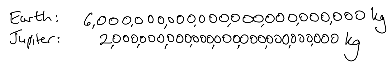
The teacher could begin by asking learners if anyone knows - or can estimate - the mass of the earth.
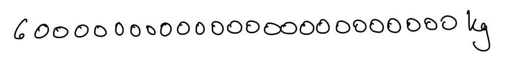
Someone might know it, but if not the teacher can write down the mass in kg. They should do this in slightly untidy handwriting, varying the sizes of the zeroes a little, as in Figure 5.8.
Jupiter is another planet in our solar system. The teacher can ask learners whether they think it is more massive or less massive than earth.
They will probably say it is more massive, because they will have in mind drawings of the solar system in which Jupiter looks a lot larger. But the teacher could remind them that size and mass are two different things. People sometimes use the word ‘massive’ to mean gigantic, but in science, massive means ‘containing a lot of mass’. Something can be larger than something else but less massive, if its mean density is less. This is an important thing to be aware of, but the purpose here is just to sow a bit of doubt.
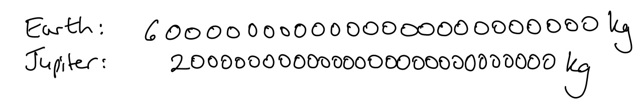
Now, the teacher writes down the mass of Jupiter, underneath the mass of the earth, but again in an untidy fashion, deliberately avoiding lining up the digits, as shown in Figure 5.9.
Now, which planet do learners think has the greater mass?
They may realise that the teacher is trying to trick them by bunching up the digits in Jupiter. But, on the other hand, they may think this is a double bluff, to try to make them think that Jupiter is more massive, when the opposite is true!
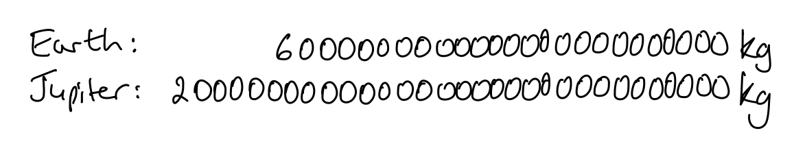
The important thing of course is not the answer. The teacher can ask the learners what would help to answer the question with more certainty. They will probably suggest lining up the digits more carefully, and making them equal sized, as in Figure 5.10, or perhaps inserting commas every \(3\) digits from the right-hand end of each number, as in Figure 5.11.
Now, what do learners think?
They will probably now say that Jupiter is more massive.
The teacher can be provocative here, by pointing at the leading digits and saying “Earth is \(6\)-something, but Jupiter is only \(2\)-something”.
Learners will articulate that the \(6\) and the \(2\) are less important than the ‘something’ - namely, the number of digits. To tell roughly how large a number is, the number of digits is more informative than the leading digit. The leading digit makes a difference only if the number of digits is the same.
Now, the teacher can ask, “How much more massive is Jupiter than the earth?”
An estimate around \(200\)-\(300\) would be good. If learners are not sure, this could be left for a moment.
The teacher could ask, “How do you think I remembered how to write down these numbers? Do you think I remembered six-zero-zero-zero-zero-zero…”. Of course, the teacher remembered for earth ‘\(6\) followed by \(24\) zeroes’ and for Jupiter ‘\(2\) followed by \(27\) zeroes’. (This might be a good moment to mention that these values are not exact, but are both rounded to \(1\) significant figure.)
This separation into ‘number between \(1\) and \(10\)’ and ‘number of zeroes’ is exactly the structure of standard form. This can often seem an arbitrary separation to learners, but by introducing it in this way it seems a completely natural way of handling large numbers, and exactly what the learners would invent for themselves.
We write ‘\(1\) followed by \(24\) zeroes’ as \(10^{24}\), so the mass of the earth is \(6\) times that, so is \(6 \times 10^{24}\) kg, and similarly the mass of Jupiter is \(2 \times 10^{27}\) kg. Learners can think of \(6 \times 10^{24}\) as beginning with \(6\) and multiplying it by \(10\) a total of \(24\) times, creating a number that is a \(6\) followed by \(24\) zeroes.
It is much easier to compare large numbers when they are written in standard form.
Now we can return to considering how many times as massive Jupiter is compared with the earth.
We can write
\[2 \times 10^{27} = 2 \times 10^{3} \times 10^{24} = 2000 \times 10^{24}.\]
Now, it is easier to compare this number with \(6 \times 10^{24}\), and we can see that the multiplier (Chapter 1) is \(\dfrac{2000}{6}\), which is about \(300\). Jupiter’s mass is about \(300\) earth masses.
The mass of the sun is about \(2 \times 10^{30}\) kg, so how much more massive is the sun than Jupiter?
This time, the \(2\)s match, and the only difference is in the power of \(10\).
Learners may say ‘\(3\) times’, because \(30 - 27 = 3\), but this \(3\) is three orders of magnitude, corresponding to \(1000\) times.
We can write \[\frac{2 \times 10^{30}}{2 \times 10^{27}} = \frac{10^{30}}{10^{27}} = 10^{3} = 1000.\] Standard form is also extremely useful for very small numbers, between \(0\) and \(1\).23
It so happens that the mass of a proton is about \(2 \times 10^{- 27}\) kg, which contrasts with the \(2 \times 10^{+ 27}\) kg value for the mass of Jupiter. Instead of starting with \(2\) kg and multiplying by \(10\) a total of \(27\) times, we begin with a mass of \(2\) kg, but divide by \(10\) a total of \(27\) times.
There is often here the same confusion with negative powers of \(10\) that we encountered in Chapter 1, where learners think that, because the power \(10^{1}\) is written as \(10\), or \(10.0\), the power \(10^{- 1}\) should be written as \(0.01\), rather than as \(0.1\).
This is really just caused by the convention that we put the decimal point to the right of the \(1\)s column, rather than (say) above it. Everything in Figure 5.12 is perfectly symmetrical about \(10^{0}\), except for the position of the decimal point! It is worth discussing this, as otherwise learners will often worry that they are ‘one out’ with the negative powers, and be unsure why.

Learners will need to master adding and subtracting numbers in standard form, even though standard form is very much designed for multiplication and division rather than addition and subtraction.24
5.5.4 Fermi problems
Fermi problems are named after the physicist Enrico Fermi, who was highly skilled at making approximate, order-of-magnitude calculations. His colleague, the physicist Richard Feynman, boasted about being able to solve in \(60\) seconds any problem that could be stated within \(10\) seconds to within \(10\%\) accuracy, although he did not always succeed.25
The intention is to make a really crude, first-order approximation, and in many situations, such an estimate is often good enough.
Learners can be very creative in inventing problems of this kind.
Here are some examples of the kinds of problems they might devise:
- Estimate how long a toilet roll would be if completely unwound.
- How long is a ball of string?
We don’t want to unwind it to measure it, as it would be difficult to get it neatly wound up again.26 - “The wheels on the bus go round and round”, but how many times on a typical journey to school?
What about the wheels on a bicycle? - In a competition, people have to guess how many sweets there are in the jar shown below.
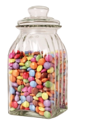 Can you make an educated estimate?
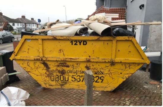
 - A \(12\)-yard skip has a maximum permitted mass of \(8\) tonnes.
Does the skip pictured below exceed that?
- How far do a pair of trousers travel when being washed in the washing machine?
Do they go further or less far when being tumble dried? - A TV news bulletin contains about \(3\) words per second.27
How does this compare with the amount of information in a typical newspaper article? - How many \(£1\) coins would you need to stack to reach the top of Mount Everest (about \(8800\) m)?
How big a container would you need to put them in afterwards?
How many lorries would you need to transport them? - If you laid down all the people in the world, end to end, how far would they stretch?
What if you put each person in a room \(5\) m \(\times\) \(5\) m \(\times\) \(5\) m?
How much space would all these rooms occupy?
Learners will initially need some help and encouragement to make sensible decisions. Typically, at the start, learners worry too much about details that will make little difference to the final answer. They may say, “But I don’t know how big a bus wheel is”. But the teacher can reply, “Have you ever seen a bus?” Learners know more than they think they do!
One strategy is to ask one learner to show a size, such as the diameter of a bus wheel, with their hands, while another learner uses a tape measure to measure the distance. With experience, learners will get better at plucking a reasonable value ‘out of the air’.
Another strategy with learners who are ‘stuck’, is to ask them to make a list of all the information they think they need to solve the problem and say next to each piece of information how important it is that they know it. Often, when they do this, the list is not actually very long, and perhaps contains just one item, which they then concede they don’t really need. Other things might be added, but then are crossed out, as learners realise they are not necessary, or are easily guesstimated.
It is possible to build up estimation problems into more of a complete modelling problem by providing a bit of a story context, giving some purpose as to why the estimate is needed. Knowing the purpose helps learners make decisions about how accurately they need to do the estimating and what assumptions are reasonable.
Here is an example of a more complete estimation task:
Alec works in a Chinese restaurant on Saturday afternoons.
He has been making prawn crackers since lunchtime and they now fill a cardboard box.
His manager asks him roughly how many he has made.
He didn’t count them, and he doesn’t want to take them out of the box to count them, as it will take a long time and they will easily break.
Instead, he photographs the box on his phone and sends it to you.
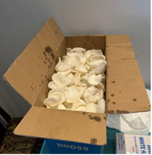
Can you help him estimate how many crackers there are?
One approach is to think of the box as consisting of layers of crackers, and estimating the number of layers and the number in each layer, perhaps by counting the number of visible crackers at the top and halving, to take account of the fact that we can see crackers that are underneath the top layer.
Another approach is to estimate the volume of the box (fairly easy) and of a single cracker (difficult) and do a division.
Another approach Alec could take would be to weigh one cracker, weigh the full box, and find a similar but empty box and weigh that too. (Weighing \(10\) crackers and calculating the mean weight would improve the accuracy.) This could be feasible in the real scenario, but would not be possible for learners to do without having access to these things.
5.5.5 Squeezing estimates between bounds
For some purposes, knowing that something is ‘about \(6\)’ may be sufficient. But more often we want to be ‘more definite’ about our estimates than that, even if we are not being particularly precise. Often, we want to be able to say ‘definitely less than \(6\)’ or ‘definitely more than \(6\)’, or make a statement like ‘definitely somewhere between \(5\) and \(7\)’. This gets us back to the supposed ‘definiteness’ of mathematics. We make some \(100\%\) true statements about a value which we are only estimating! This builds on work on inequalities (Chapter 2), which in real situations can be much more prevalent than exact equations.28
The following task offers a way into thinking about this:
A thermostat digital display constantly flickers between \(17 ^\circ\text{C}\) and \(18 ^\circ\text{C}\).

What can you conclude from this?
Learners might conclude that the temperature must be around \(17\text{-18} ^\circ\text{C}\), which would be reasonable.
But can we say more than that? Why would the temperature keep switching back and forth between these two numbers every second or so, rather than remain on one of them?
Learners often respond that the temperature must be close to \(17.9 ^\circ\text{C}\), but actually it must be very close to \(17.5 ^\circ\text{C}\), as this is the temperature right on the boundary between temperatures that round down to \(17 ^\circ\text{C}\) and up to \(18 ^\circ\text{C}\). If the temperature were close to \(17.9 ^\circ\text{C}\), the display would just show \(18 ^\circ\text{C}\) constantly.
Upper and lower bounds are really just the inverse problem to rounding. We have a number that has already been rounded – and we want to discover what the exact number might have been.
Lower bounds are a lot simpler than upper bounds, so it helps to begin there.
A number rounds to \(18\) to the nearest integer.
What might the number have been?
It may take a few seconds for learners to realise that the answers to this question will be \(decimals\), and not integers.
As always, drawing a number line going up in whatever we are rounding to (\(1\)s in this case) is helpful. Then we can see that the values of \(x\) that round to \(18\) are \(17.5 \leq x < 18.5\).
In Figure 5.13, I have coloured in \(17.5\), to show that it is included, but left \(18.5\) as an open circle, to show that it is excluded. Every value up to, but not including, \(18.5\) is included.

While learners may not have too much trouble with \(17.5\) being the lower bound, there is always a lot of difficulty over \(18.5\) being the upper bound. After all, \(18.5\) is the lower bound of \(19\), so how can it be both a lower bound and an upper bound? I think we can just be honest and say that it is indeed a bit unsatisfactory, but any number other than \(18.5\) would definitely be a wrong choice for the upper bound of \(18\).
Learners often think that the upper bound should be \(18.4\), but that would exclude \(18.41\), \(18.42\), and so on, which are all greater than \(18.4\) but round down to \(18\). So, \(18.4\) isn’t large enough to be the upper bound of \(18\).
Then, learners might instead suggest using \(18.49\), but again, that would exclude \(18.491\), \(18.492\), and so on. This is going to happen however many \(9\)s we put on the end: \(18.499,999,99\) would exclude the numbers \(18.499,999,991\), \(18.499,999,992\), and so on.
The only way in which we can say ‘up to but not including \(18.5\)’ is to say ‘up to but not including \(18.5\)’. There is no highest number less than \(18.5\) that we can name; whatever number less than \(18.5\) we think of, there will always be infinitely many higher ones that are still less than \(18.5\). University mathematics students studying Analysis find this difficult, so there is no reason to expect that learners in school will not!29
We will take the example calculation from Section 5.5.3.2, and, rather than just estimating it to be ‘about \(1\)’, obtain some bounds on the value.
The exact quantity was
\[x = \frac{\sqrt{51.3} + 1.48}{13.7 - 5.62}.\]
To find an upper bound for \(x\), we can replace the numbers in the numerator by the next highest convenient values, to give \(\sqrt{64} + 2\).
To obtain an upper bound for \(x\), we need the denominator to be as small as possible.
So, we need to round \(13.7\) down and \(5.62\) up, since that will make the difference between them as small as it can be.
We obtain \[\text{upper}(x) = \frac{\sqrt{64} + 2}{13 - 6} = \frac{8 + 2}{7} = \frac{10}{7} ,\] or about \(1.4\) (rounding up).
The opposite process to find a lower bound gives
\[\text{lower}(x) = \frac{\sqrt{49} + 1}{14 - 5} = \frac{7 + 1}{9} = \frac{8}{9} ,\]
or about \(0.8\) (rounding down).
So, we can conclude \(0.8 < x < 1.4.\)
We can be completely sure that whatever the exact value of \(x\) is, it cannot be less than \(0.8\) or greater than \(1.4\), so it must lie within this interval.
The exact answer was \(x = 1.06960418\ldots,\) which is well inside the interval.
It is easy to situate problems like this in real-world contexts.30
5.5.6 Making judgments
Sometimes the purpose of an estimation is to produce an informative number. But on other occasions the purpose of an estimation is to make a decision or a judgment, such as whether you have enough money or not to buy something, or whether some claim is plausible or implausible. The end product here is ‘yes/no’ or ‘buy/sell’ or ‘believe/don’t believe’, and so on, rather than a numerical answer.
Many problems like this are set in a context of purchases of one kind or another:31
Which offer below will save you the most money?

Learners can conclude that ‘Half price’ is always preferable to ‘\(30\%\) off’, because half price is equivalent to \(50\%\) off, which is a greater saving. However, whether the other deals are better or worse depends on other factors. For example, \(£12\) off is better than half price, if the item costs less than \(£24\), but worse if the item costs more than \(£24\).
Learners may think that ‘Buy one, get one free’ is equivalent to ‘Half price’, but this is not necessarily the case. ‘Buy one, get one free’ is only beneficial if the buyer wants two items, or can sell or somehow make use of the second one. They also need to have enough money to pay the normal price, otherwise this may not be an option for them.
Learners could invent other special offers to compare.
A different kind of decision task is to assess a proposed approximation to see whether it is likely to be good enough to be useful in practice:
The Tailor’s Rule of Thumb is a simple approximation used by tailors to estimate the wrist, neck and waist circumferences of someone, based on just one measurement of the circumference of their thumb:
\[
\begin{matrix}
\text{thumb} & \fixedarrow{$\times 2$} & \text{wrist} & \fixedarrow{$\times 2$} & \text{neck} & \fixedarrow{$\times 2$} & \text{waist.} \\
\end{matrix}
\]
Each measurement in the rule is of the circumference of that part of the body.
Why/when might this approximation be convenient in practice?
Investigate how accurate it is.
Would it be worth obtaining more precise values for the multipliers than \(2\)?
Being measured for clothes could be time-consuming and inconvenient. It could also entail someone leaving their home and attending a shop. So, learners will be able to see that this simple rule might be very welcome, provided it works well enough in practice. Clothes don’t have to fit with millimetre precision, so maybe the rule is good enough?
Typically, learners think that \(2\) seems too small a multiplier for some or all of these relationships, and there is much scope for checking with a tape measure. It may seem too good to be true that all the multipliers are close enough to the same value, \(2\), and learners could investigate which relationships are least well modelled in this way.
If they could change just one of the multipliers to something more accurate, which one would they change?
Do the errors accumulate the more times the rules are used? For example, is the error in predicting waist measurement from thumb measurement worse than in predicting neck measurement from thumb measurement?
Does the rule work better for some kinds of people than others?
A common kind of decision task is to be presented with a claim and be asked to decide whether it is believable or not. This is a key skill everyone should have for consuming news media, for example.
Learners repeatedly arrive late for their school mathematics lesson.
The teacher claims, “If everyone were \(5\) minutes late to every mathematics lesson, that would add up to \(3\) weeks of lost learning every year!”
Is this claim credible?
It may not be quite clear what exactly the teacher is claiming.
We could suppose there are \(200\) school days in the year, with a single \(1\)-hour mathematics lesson every day.
Losing \(5\) minutes from each lesson would add up to \[200 \times 5 = 1000 \text{ minutes},\] which is \[\frac{1000}{60} \text{ hours},\] or about \(17\) hours.
This is about \(3\) weeks of lessons, so the claim could be reasonable.
But perhaps ‘\(3\) weeks of lost learning’ suggests \(15\) days of entire mathematics lessons, which would be considerably more.
On the other hand, if there are \(30\) learners in the class, perhaps the time lost should be multiplied by \(30\), which would make \(90\) weeks of lessons, which is more than twice a school year!
As it stands, the statement may be credible, but there are other ways to frame the situation.
A loss of \(5\) minutes is a loss of \(\dfrac{1}{12}\) of a lesson, which is a bit less than \(10\%\). This is true regardless of the number of lessons. Does presenting it this way make the lateness seem less serious or more serious?
Another task focused on believability is this one:
This is what they say:
| Mr T: | I’m \(10^{9}\) seconds old. |
| Ms P: | I’m \(9999\) days old. |
| Ms C: | I’m \(10^{4}\) weeks old. |
| Mr R: | I’m \(500\) months old. |
| Mrs N: | I’m \(200,000\) hours old. |
| Ms L: | I’m \(20,000,000\) minutes old. |
Which person is definitely mistaken?
Work out the ages of the other teachers in years.
Rounding down (because it is age) to the nearest year below, the ages come to \(31\) years, \(27\) years, \(191\) years, \(41\) years, \(22\) years and \(38\) years. So, Ms C must be mistaken.
A related task is this one:
Work out how many seconds it is until you…
…have lunch.
…go home.
…go to bed.
…start the holiday.
…finish compulsory education.
Learners could estimate first ‘off the top of their head’, and then calculate and see how close they were.
Here is another decision-focused task that requires estimation:
Laura says, “At the weekend, I’m going to count up to a million.”
Aga says, “That’s impossible! No one lives long enough to count up to a million!”
Who is correct?
Learners might notice that Laura doesn’t specify that she counts ‘in ones’! If she counts up in hundreds, say, how much difference would that make?
Learners often begin by assuming that each number will take perhaps \(1\) second to say.
This leads to converting: \[10^{6} \text{ seconds} = \frac{10^{6}}{60} \text{ minutes} = \frac{10^{6}}{60^{2}} \text{ hours} = \frac{10^{6}}{24 \times 60^{2}}\text{ days},\] which is about \(12\) days.
This assumes no sleep or breaks, so a more reasonable answer might be \(2\) or \(3\) times as long as this. Certainly, Laura won’t have time to count up to a million ‘at the weekend’, but perhaps she could do it over a long holiday.
One number per second might be reasonable for smallish numbers, but by the time Laura is counting numbers like “four hundred and sixty-five thousand three hundred and ninety-four”, she will certainly take longer than \(1\) second.
So, a more sophisticated estimate might involve assigning different mean times for different sizes of number. Learners could use stopwatches to help them find suitable values, such as those shown below.
\[ \begin{array}{cc} \hline \text{Number range} & \text{Estimated time per number (seconds)} \\ \hline 1{-}100 & 1 \\ 101{-}999 & 2 \\ 1001{-}9999 & 2 \\ 10,001{-}99,999 & 3 \\ 100,001{-}1,000,000 & 4 \\ \hline \end{array} \]
Using these values, the total number of seconds will be about
\[1 \times 100 + 2 \times 900 + 2 \times 9000 + 3 \times 90,000 + 4 \times 900,000= 3,889,900.\]
This is nearly four times as long as the ‘\(1\) second per number’ estimate, because most of the numbers are greater than \(100,000\), and therefore are assigned \(4\) seconds. Because of this, learners may conclude that using the values in the table above was unnecessary, and that we should have just estimated \(4\) seconds for every number.
Four million seconds will be about four times as long as \(12\) days, so we might estimate about \(50\) days, which would be longer if Laura wanted to take breaks for sleeping, eating and resting her voice.
Would you rather earn \(£1\) per second or \(£1\)m per week?
A week is \(60 \times 60 \times 24 \times 7 = 604,800\) seconds, taking a week as \(7\) days, and so earning \(£1\) per second would generate \(£604,800\). This is less than \(£1,000,000\), so \(£1\)m/week is a higher salary.
5.6 Probability
Although it is possible to pose probability problems in a purely mathematical context, such as asking for the probability of obtaining a prime number when selecting at random a number from the positive integers less than \(100\), most of the time probability tasks are to do with the real world.
5.6.1 The nature of probability
Probability is all about quantifying uncertainty, or risk.
In everyday life, we often use words like ‘probably’, ‘certain’ or ‘unlikely’. In mathematics, we use the words ‘certain’ and ‘impossible’ very frequently, and we mean those as absolutes. It is certain that Pythagoras’ Theorem is true; it is impossible to find a multiple of \(6\) which is odd.
We can think of probability as considering all the statements that lie between these extremes of certainty (probability \(= 1\)) and impossibility (probability \(= 0\)). It is in between these values on a probability scale that, in practice, all real-life statements are to be found (Figure 5.14).

We might place words such as ‘likely’ on this scale, but they don’t have exact locations. We might call the midpoint, with probability \(0.5\), ‘even chance’ or ‘fifty-fifty’, but to describe any other locations along the scale precisely, we will need to use numbers.
We often emphasise to learners that other scales that we represent on number lines go on forever in both directions. For example, learners may think of fractions as having to lie between \(0\) and \(1\), but improper fractions (e.g. \(\frac{11}{4}\)) or mixed numbers (e.g. \(2\frac{3}{4}\)) can be greater than \(1\), and negative fractions can take any negative value.
However, the probability scale is a number line which really does absolutely stop at its ends. A probability cannot be less than zero or greater than \(1\). Nothing can be less likely than impossible or more likely than certain. (Another example of a finite number line is the strictly \(- 1\) to \(1\) scale for correlations - see Chapter 4.)
Because we are talking about uncertainty, learners often think that probabilities are approximate, but they are no more approximate than any other values in mathematics.32 What is uncertain is whether an event will happen or not. But we might nevertheless be completely certain about its probability of happening.
For probabilities of zero or \(1\), we know that the event will never or always happen. However, for probabilities in between these extreme values, we cannot know on any specific occasion whether the event will or will not happen. But we might know for sure that the probability is, say, precisely \(60\%\).
For example, if we select an integer at random from the first \(5\) positive integers, there is an exactly \(60\%\) chance of our integer being less than \(4\), because exactly \(\frac{3}{5}\) of those available integers are less than \(4\).
Figure 5.15 shows the entire possibility space (also called sample space) for the trial in which we randomly select our integer: the possibility space contains all the possible outcomes that can happen.
\[ \require{colortbl} \begin{array}{|c|c|c|c|c|} \hline \cellcolor{#D3D3D3} \rule{0pt}{4ex} \rule[-2.5ex]{0pt}{0pt} \hspace{2.15em} 1 \hspace{2.15em} & \cellcolor{#D3D3D3} \hspace{2.15em} 2 \hspace{2.15em} & \cellcolor{#D3D3D3} \hspace{2.15em} 3 \hspace{2.15em} & \hspace{2.15em} 4 \hspace{2.15em} & \hspace{2.15em} 5 \hspace{2.15em} \\ \hline \end{array} \]
If we call the integer we select \(x\), then the possibility space shows all the possible values of \(x\) that can be obtained.
An event is any subset of the possibility space.
For example, the event \(A\) could be ‘\(x < 4\)’, shown shaded in Figure 5.15.
In situations in which symmetry tells us that the outcomes are equally likely, we can be precise about the probabilities of events. Because each of the five numbers is equally likely to be selected, the probability of selecting any one of them must be \(\frac{1}{5}\) of the possibility space, and so the probability of event \(A\) is \[\frac{1}{5} + \frac{1}{5} + \frac{1}{5} = \frac{3}{5}\] of the entire possibility space, or \(\frac{3}{5}\) (the shaded fraction in Figure 5.15).
The reason we can add together the three probabilities (\(\frac{1}{5}\), \(\frac{1}{5}\) and \(\frac{1}{5}\)) to find the probability of \(x\) being either \(1\) or \(2\) or \(3\) is that the three outcomes (\(1\), \(2\) and \(3\)) in our possibility space were not only equally likely but mutually exclusive, meaning that more than one of them cannot happen simultaneously. The three outcomes are distinct and non-overlapping, so we find the total amount of probability space they cover by adding up the amount of space covered by each one.
We use the notation \(P(A)\), like the function notation \(f(x)\), to mean ‘the probability of’ an event \(A\), so here we can write
\[\begin{array}{rcccccccc} P(A) & = & P(x < 4) & = & P(x = 1) & + & P(x = 2) & + & P(x = 3) \cr \cr & & & = & \dfrac{1}{5} & + & \dfrac{1}{5} & + & \dfrac{1}{5} \cr \cr & & & = & \dfrac{3}{5}. \end{array}\]
While the individual, separate outcomes in a possibility space are always mutually exclusive, more generally, events aren’t necessarily. The events ‘\(x<4\)’ and ‘\(x<5\)’ are not mutually exclusive. Neither are the events ‘\(x<4\)’ and ‘\(x>2\)’. In each case, the events overlap - they contain some common outcomes.
Learners often work out basic probabilities like this by writing ‘the total number of outcomes’ as the denominator and ‘the number of desired outcomes’ as the numerator, but are often unclear why those numbers go in those positions. I think it can be helpful to understand the probability of an event such as \(P(A)\) here as the sum of the probabilities of three individual outcomes, i.e., \[\frac{1}{5} + \frac{1}{5} + \frac{1}{5} = \frac{3}{5}.\]
Let’s consider another event \(B\), which is the event ‘\(x\ =\) a prime number’.
The prime numbers in our possibility space are \(2\), \(3\) and \(5\), so \[P(B) = \frac{1}{5} + \frac{1}{5} + \frac{1}{5} = \frac{3}{5} \text{ also.}\]
(Learners may need reminding that \(1\) is not prime.)
But the probability of ‘\(A\) or \(B\)’ happening, which we write as \(A \cup B\) (\(A\) union \(B\)), is not \[P(A) + P(B) = \frac{3}{5} + \frac{3}{5} = \frac{6}{5}.\] That is obviously wrong, because \(\frac{6}{5} > 1\), and no probability can be greater than \(1\).
The reason we cannot add the probabilities of these two events to find the probability of either of them happening is that these events \(A\) and \(B\) are not mutually exclusive. They can both happen simultaneously.
For example, if \(x = 2\), then \(A\) has happened and \(B\) has happened, because \(2\) is both less than \(4\) and also prime, so \(2\) is included in both events, but it is still just the same \(2\), so we must not double-count it. If we just add up \(P(A)\) and \(P(B)\), we include an outcome like \(2\) twice.
Figure 5.16 shows that outcomes \(2\) and \(3\) are common to both events.
\[ \require{colortbl} \begin{array}{cl} A & \begin{array}{|c|c|c|c|c|} \hline \cellcolor{#D3D3D3} \rule{0pt}{4ex} \rule[-2.5ex]{0pt}{0pt} \hspace{2.15em} 1 \hspace{2.15em} & \cellcolor{#D3D3D3} \hspace{2.15em} 2 \hspace{2.15em} & \cellcolor{#D3D3D3} \hspace{2.15em} 3 \hspace{2.15em} & \hspace{2.15em} 4 \hspace{2.15em} & \hspace{2.15em} 5 \hspace{2.15em} \\ \hline \end{array} \\ \\[-1ex] B & \begin{array}{|c|c|c|c|c|} \hline \rule{0pt}{4ex} \rule[-2.5ex]{0pt}{0pt} \hspace{2.15em} 1 \hspace{2.15em} & \cellcolor{#D3D3D3} \hspace{2.15em} 2 \hspace{2.15em} & \cellcolor{#D3D3D3} \hspace{2.15em} 3 \hspace{2.15em} & \hspace{2.15em} 4 \hspace{2.15em} & \cellcolor{#D3D3D3} \hspace{2.15em} 5 \hspace{2.15em} \\ \hline \end{array} \end{array} \]
We write the overlap between two events \(A\) and \(B\) as \(A \cap B\) (\(A\) intersection \(B\)).
To find the probability of \(A \cup B\), we could add the probabilities for \(A\) and \(B\), provided we also then subtract the probability for \(A \cap B\), in order not to double-count the event \(A \cap B\):
\[P(A \cup B) = P(A) + P(B) - P(A \cap B)\]
\[= \frac{3}{5} + \frac{3}{5} - \frac{2}{5} = \frac{4}{5}.\]
We can see this is correct, because the probability of randomly selecting a number that is either less than \(4\) or is prime is equal to the probability of selecting \(1\), \(2\), \(3\) or \(5\), which consists of \(4\) equally-likely outcomes out of \(5\) altogether, giving a probability of \(\frac{4}{5}\).
The natural way to represent non-mutually exclusive events is as overlapping circles on a Venn diagram, as in Figure 5.17.33

We can see ‘by colouring in’ that the region in which either \(A\) or \(B\) happens (\(A \cup B\)) is less than the sum of the discs corresponding to \(A\) and\(\ B\), because of the overlapping, intersection region (\(A \cap B\)).
So, if we want to count each region once only,
\[P(A \cup B) = P(A) + P(B) - P(A \cap B) ,\]
where the \(- P(A \cap B)\) term removes the part that was double-counted.
This may seem like a complicated formula to introduce early on in learning about probability, but I think the longer it is delayed the more confusions can arise around vague statements like “‘and’ means multiply, and ‘or’ means add”.
Learners are sometimes confused by this formula, thinking that the probability of ‘\(A\) or \(B\)’ happening, \(P(A \cup B)\), does not include the probability that they both happen, and that is why we need to subtract \(P(A \cap B)\), which is the probability that both \(A\) and \(B\) happen.
However, ‘or’ in mathematics is always inclusive, so \(P(A \cup B)\) does mean the probability that either \(A\) or \(B\) happens, or both.
We subtract \(P(A \cap B)\) because in \(P(A) + P(B)\) the ‘both’ region has been counted twice, once within \(P(A)\) and once within \(P(B)\), and the subtraction removes the unnecessary second counting of \(P(A \cap B)\).
If we wanted the probability that either \(A\) or \(B\) happens, but not both, known as the exclusive or or symmetric difference, \(A \mathbin{\Delta} B\), then we would have to subtract \(P(A \cap B)\) twice, so \[P(A \mathbin{\Delta} B) = P(A) + P(B) - 2P(A \cap B).\]
To represent mutually exclusive events in a Venn diagram, we either draw the circles as not overlapping each other (Figure 5.18), or we use the same overlapping diagram as in Figure 5.17, but just state that the overlapping region is empty.

If \(A\) is the event ‘\(x < 4\)’, then we can use the notation \(A'\) to indicate the complement of this event; i.e., the event ‘\(A\) doesn’t occur’. So, the event \(A'\) is ‘\(x \nless 4\)’ or, equivalently, ‘\(x \geq 4\)’.
An event and its complement are always mutually-exclusive, meaning they can’t both happen on any particular trial. A number cannot be less than \(4\) and also not less than \(4\).
Learners sometimes think that \(4\) itself might be neither \(A\) nor \(A’\), but \(4\) is not less than \(4\), because it is equal to \(4\), so it is in \(A'\), not \(A\).
Not only are an event and its complement mutually exclusive, they are also mutually exhaustive, meaning that, taken together, they cover all of the possibilities. Either \(A\) must happen or \(A’\) must happen; if \(A\) doesn’t happen, then \(A’\) must happen, and vice versa.
So, \[P(A) + P(A') = 1.\]
A consequence of this is that, when you want to know \(P(A)\), sometimes it is easier to work out \(P(A')\) and then calculate \(P(A) = 1 - P(A')\).
For example, when working out \(P(A \cup B)\) above, we might notice that the only way in which \(A \cup B\) can not happen is if \(x = 4\), because \(4\) is the only one of these integers which is not less than \(4\) and is also not prime. It follows then that \[P(A \cup B) = 1 - P\left( (A \cup B)' \right) = 1 - \frac{1}{5} = \frac{4}{5},\] as before.
A very common misconception in probability is to assume that an event and its complement must be equally likely.
We can see that \(P(A) = \frac{3}{5}\), which is more than \(\frac{1}{2}\), and therefore \(P(A')\) must be less than \(\frac{1}{2}\), so that they can sum to \(1\). So, \(P(A)\) and \(P(A')\) certainly cannot be equal.
In everyday life, people will sometimes use the language of ‘It’s fifty-fifty’ to mean ‘There are two choices’, rather than ‘There are two equally probable choices’. Often complementary alternatives are very far from equally likely. Tomorrow, I might receive an unsolicited gift of \(£1\)m, or, on the other hand, I might not. These are two possible, mutually-exclusive and exhaustive complementary outcomes. But unfortunately, not receiving \(£1\)m is considerably more likely!
Lots of aspects of probability can be counterintuitive, and even experts are often wrong on sometimes seemingly basic-sounding questions. In other areas of mathematics, we encourage learners to estimate an answer before calculating, and check their answer is of a sensible size. But often with probability calculations it can be very hard to say whether a probability of, say, \(\frac{2}{7}\), is ‘about the right size’ or not.
5.6.1.1 Frequentist probability
It is important to discuss with learners what a probability of, say, \(60\%\) really means, as otherwise they will always feel that probability is a mysterious topic.
In a frequentist understanding of probability, a probability is the long-run relative frequency of something happening. An event with a probability of \(60\%\) will happen on \(60\%\) of occasions, in the long run.
The number of times it happens, expressed as a fraction of the number of times it could have happened, is the relative frequency. This value will get arbitrarily close the ‘true’ probability as the total number of trials increases, meaning that we can get as close as we like to the true probability by conducting enough trials.
An example I like to use, and find more useful than coins, is a drawing pin, because these come in different makes and sizes. Like a coin, when thrown a drawing pin can land ‘heads’ or tails’ (Figure 5.19).

However, unlike a coin, there should be no expectation that heads and tails will necessarily be equally likely. It is surprising, but although you can make a biased die, you cannot really have a biased coin, unless it is a double-head or double-tail coin - at least if you are going to flip it (as opposed to spin it on a table).34
Is a thrown drawing pin more likely to land heads or tails? Why?
Learners will often think that because there are two outcomes, they must be equally likely. However, it is intuitive that really this must depend on the details of the particular drawing pin.
Imagine a drawing pin that had a much smaller rounded section and a longer pin, such as the one shown in Figure 5.20.

It would surely be very unlikely for this design of drawing pin to land tails, and it would be much more likely to land heads. Balancing as tails would be quite unstable, and the drawing pin would be very likely, with the slightest bump or gust of air, to topple over into heads.
If learners disagree, just make the pin more extreme, with an even longer straight part, so that it becomes more like a nail (Figure 5.21). No one will expect this to land tails.

To find the probability of any particular design of drawing pin landing heads, we could do either of two things:
Make careful measurements of the drawing pin’s features, such as the length of the straight part, and the radius of curvature of the head part. Then, we could do some calculations based on physics/mechanics, such as finding its centre of mass to estimate its relative stability in the heads and tails positions. To do this, we would need to make assumptions, such as uniform density of the material, and so on. We could also model how the drawing pin was being thrown, and make assumptions about air resistance, spin and so on. This would give us a theoretical probability, which we would need to check out in practice to see how accurate the prediction of the probability was.
Take one of the drawing pins and throw it a large number of times. Equivalently, take a large number of identical drawing pins, throw them all at once, and count how many come up heads. Then repeat, and continue accumulating more and more data until the relative frequency settles down to some specific value. This value would be the empirical probability. This also involves making assumptions, such as that the bumping of drawing pins into other drawing pins is ‘random’, and doesn’t influence in any systematic way how they end up oriented. It also involves deciding when enough data have been collected to make a sufficiently reliable estimate of the probability.
Approach #1 would require mathematics and physics beyond the scope of school, but it is good for learners to be aware of this possible approach. They should experience doing approach #2 for themselves, to get a sense of what a frequentist probability actually means.
Qayla throws a drawing pin repeatedly, and records her results like this:

What can you conclude about her drawing pin?
Since there seem to be just two orientations in which the drawing pin can land, it is a bit tedious and unnecessary to sketch the outcome every time, like this.
Instead, we could save time by just writing:
\[ \begin{gathered} \text{HTTHH} \qquad \text{HHTHT} \qquad \text{HHTHT} \qquad \text{THTHT} \qquad \text{TTTHH} \\ \text{THHHT} \qquad \text{HHHHH} \qquad \text{HHTHH} \qquad \text{HTTHT} \qquad \text{HHHTH} \end{gathered} \]
Even simpler than this, we could just tally up how many heads and tails we get, and present the result as, say:
\[31 \text{ heads and } 19 \text{ tails.}\]
The relative frequency of heads is therefore
\[\frac{31}{31 + 19} = 0.62.\]
This means that on \(62\%\) of the throws, the drawing pin landed heads.
It is important to interpret this carefully, in the past tense. It doesn’t mean that on exactly \(62\%\) of future throws it will land heads. We never know for sure what the future holds. If we throw the drawing pin \(50\) more times, we are certainly not guaranteed \(31\) tails and \(19\) heads - it would be quite unlikely to get exactly the same numbers again. We might get \(0\) tails and \(50\) heads, or \(50\) tails and \(0\) heads, or anything in between.
However, the more trials we do, the more closely we would expect our value to converge to the ‘true’ value, which we don’t know, but is probably somewhere around \(0.62\).
Learners could work in pairs to do the throws - as many as they can record in a fixed number of minutes, or a pre-specified number. And then, on a spreadsheet, one by one the teacher can include results from more and more pairs of learners, and everyone can observe the relative frequency settling down to a value close to the ‘true’ value.
Alternatively, learners can record their results as they go, straight onto a random-walk plot, as shown blank in Figure 5.22(a) and completed in Figure 5.22(b).35 (A downloadable copy of a blank random-walk plot is available online.36)
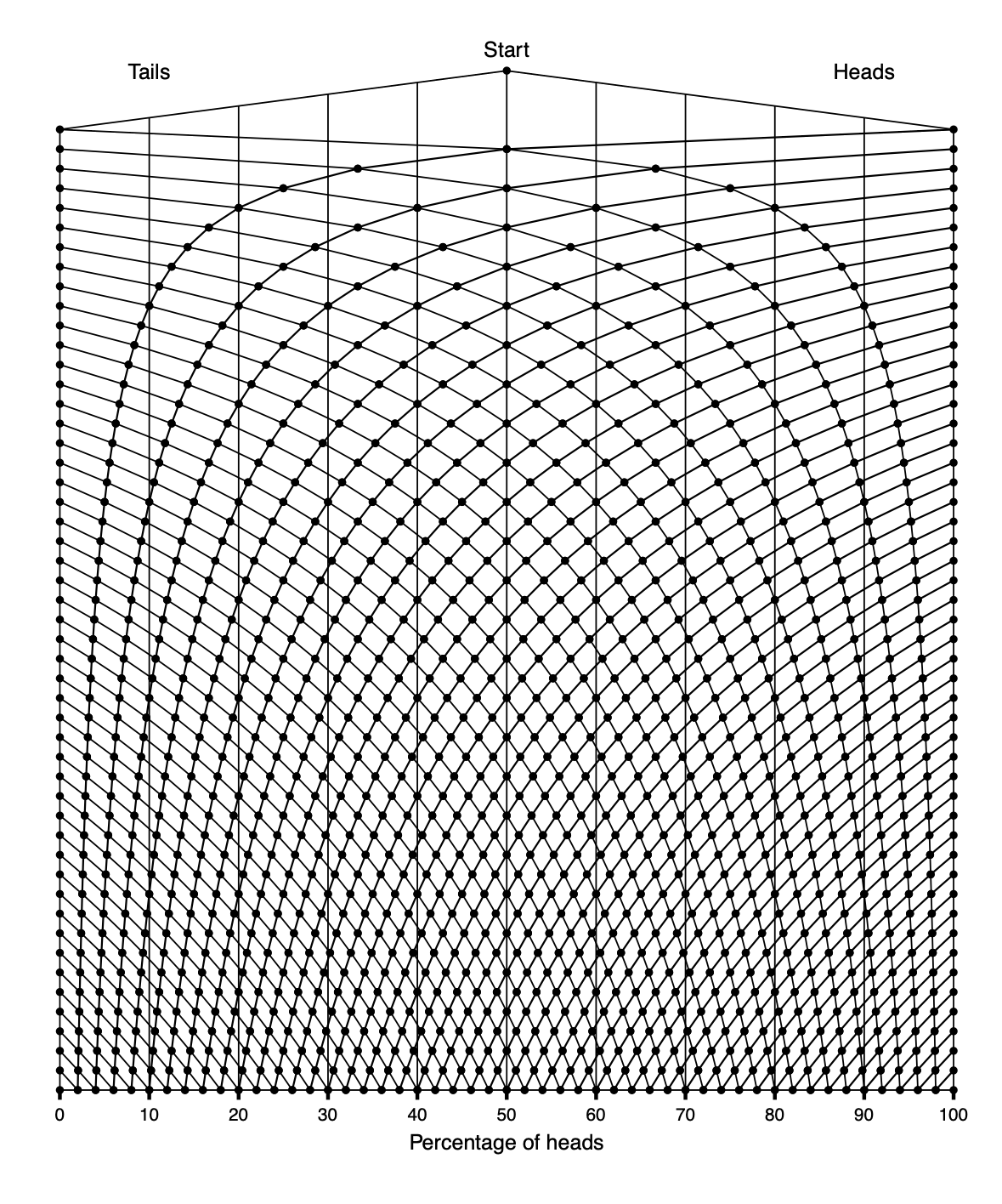
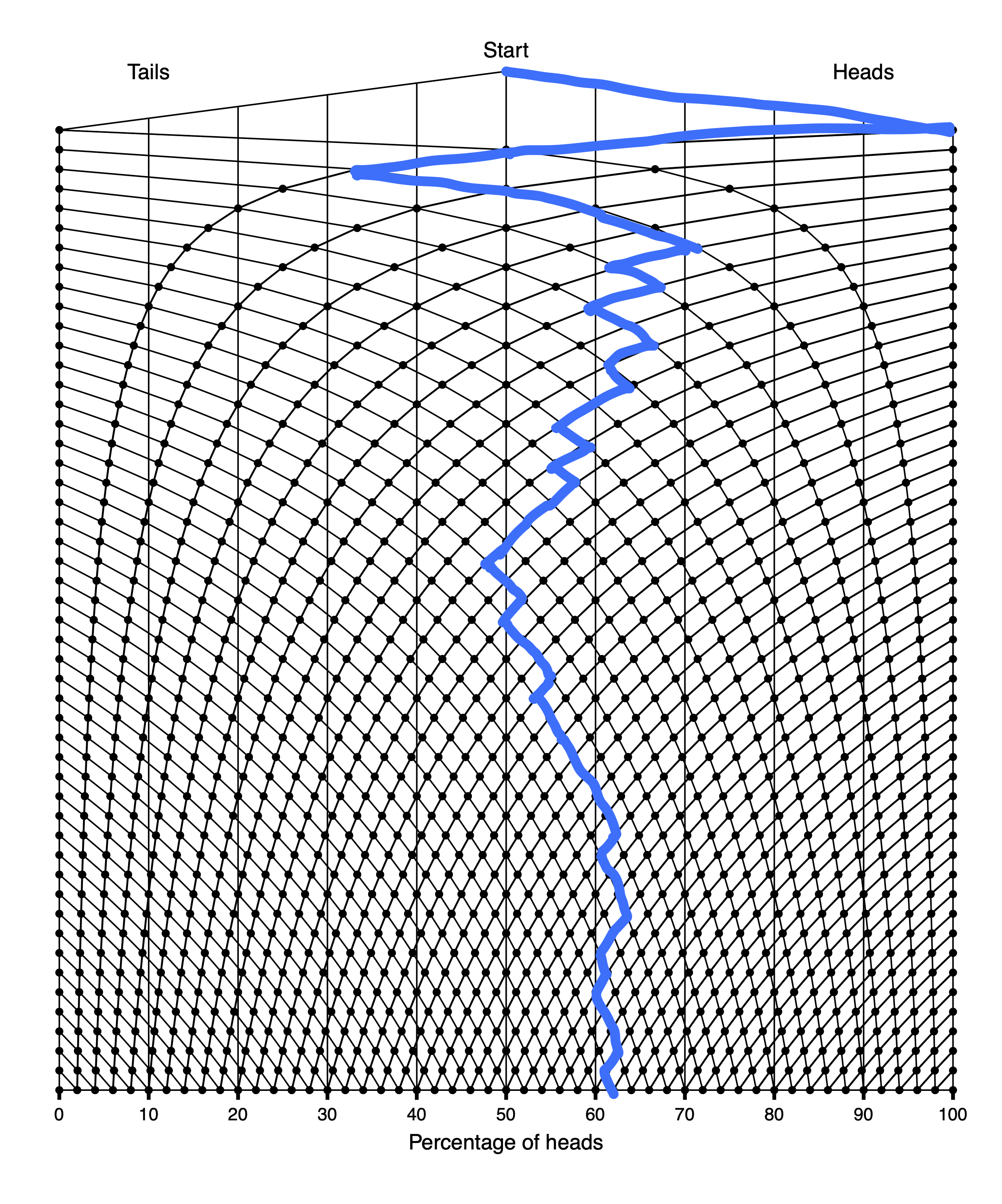
The outcome of each throw carries equal weight in pushing us either towards the left (zero probability) or towards the right (\(100\%\) probability). This means that each successive throw of the drawing pin has a smaller and smaller effect on the relative frequency calculated up to that point, which is tracked relative to the percentage scale at the bottom of the the plot. When \(50\) throws have been completed, we reach the bottom of the plot and read off the relative frequency as a percentage.
The frequentist interpretation of probability is that the probability of getting heads with this particular kind of drawing pin is the value that the relative frequencies converge to as the number of throws gets very large. The law of large numbers states that we can get as close to the true value as we wish, just by doing enough trials.
From our data, we would estimate
\[P\left( \text{heads} \right) = 0.62.\]
Equivalently, we could say
\[P\left( \text{tails} \right) = 1 - 0.62 = 0.38 ,\]
because heads and tails are complementary events.
This assumes that no drawing pin could ever land in any other orientation, such as ‘on its tip’, for example (Figure 5.23), which we might want to class differently from ‘heads’, where the edge of the rounded part is resting on the flat surface.

This is a modelling assumption and decision. For instance, we are assuming that the drawing pins are being thrown onto a hard surface. If, instead, they were landing on something more like modelling clay, many pins might land in that ‘on its tip’ orientation, and the probability of the regular kind of heads would be smaller. The probability is not really just a property of the drawing pin, but of the whole scenario - how it is thrown, onto what surface, how we choose to record the different orientations, etc.
Another good practical scenario for probability experiments, and safer than handling sharp pins, is spinners.
It is easy for learners to quickly create a spinner, by dividing a circle into sectors, placing a paper clip at the centre and trapping it with a pencil. Then, they can flick the paper clip with their finger and it will spin around the end of the pencil and stop in one of the sectors, as shown in TASK 5.24. With spinners, it is very intuitive which outcomes should be more likely and by how much, because we expect that the probability of the paper clip stopping in any sector should be proportional to the area (or angle) of that sector.
A good task to test learners’ developing sense of probability is the following:37
A spinner has a quarter-circle red and three-quarters yellow, as shown below.

You have to predict which colour the spinner will land on.
You are going to make \(20\) predictions, and on each prediction you win if you are correct.
How many of the \(20\) times will you predict red?
Many learners will calculate \(\frac{1}{4} \times 20\) and say that they will predict red \(5\) out of the \(20\) times.
But of course they should never predict red, because on every spin yellow is more likely to come up!
Even if the spinner were \(\dfrac{5}{12}\) red and \(\dfrac{7}{12}\) yellow (Figure 5.24), they should still never predict red.

I find that learners are often surprised by this, but it is never wise to predict a less likely option! Their answer of \(5\) is the right answer to a different question:
If you had to predict how many times red would be obtained in \(20\) spins, what would be your best guess?
For this task, you can’t do better than predicting \(5\) reds, because that is the mean number of times red would be obtained in \(20\) spins. However, for a question like this, if the mean is not an integer, then you will have to choose the nearest integer, because the answer has to be an integer.
5.6.1.2 Bayesian probability
A different way of thinking about probability is the Bayesian approach.
Here, by ‘probability’ we mean how sure someone ought to be that something will happen. This can apply to a broader range of situations than frequentist probability can.
For example, for the drawing pin, based on the data considered above, we might say we were about \(62\%\) sure that if we throw the drawing pin again it will land heads. So, the Bayesian probability could be the same as the frequentist probability here. The degree of certainty would depend on how much evidence had been collected and how compelling it was, and might differ from person to person.
Frequentist probabilities don’t work for events which are ‘one-offs’. When we say the probability of a certain person, say Donna, becoming an engineer when she grows up is \(80\%\), we can’t interpret this in a frequentist fashion. We can’t take a large number of ‘Donnas’ and see how many of them become engineers. To make sense of the statement in frequentist terms, we would have to imagine collecting together all the things we think are ‘\(80\%\) likely’, including Donna becoming an engineer. Then, provided there are a large number of those things, we would expect that about \(80\%\) of them would actually happen, and \(20\%\) wouldn’t. We don’t know if the statement about Donna is in the \(80\%\) or the \(20\%\), but this is the best we can do.
But Bayesian probability can apply even if there is just a single occurrence. We can talk about the Bayesian probability of a certain degree of climate change by \(2100\), for instance, or the probability that life exists on other planets in our galaxy. We can’t repeat these things lots of times and take an average, so they don’t work from a frequentist point of view.
Learners may not be expected to know terms like ‘frequentist’ or ‘Bayesian’, but these distinct ways of thinking about probability are valuable to share, otherwise learners may feel that they are encountering different things under the same heading of ‘probability’ and cannot see how they are connected.
5.6.2 Randomness
The phrase ‘at random’ or ‘selected randomly’ appears a lot in probability, and is very important, but learners are often confused about what it means, and unfortunately sometimes questions given to learners omit to mention the random aspect.
A task that could surface this is the following:
If I choose an integer from \(1\) to \(5\), what is the probability that it is prime?
This question does not mention ‘at random’, and really, as it stands, is impossible to answer. If I know which numbers are prime, then I can deliberately ‘choose’, say, \(3\), and know for certain that it is prime! This would make this question the usual style of question in mathematics: “Which of these integers are prime?”, and there is not supposed to be any guessing involved.
This contrasts with the question:
If I choose an integer from \(1\) to \(5\), what is the probability that it is greater than \(10\)?
Here, the answer obviously must be zero, since there are no numbers greater than \(10\) among the integers from \(1\) to \(5\). No matter how carefully I ‘choose’ my number, it cannot exceed \(10\), so the omission of any reference to randomness this time makes no difference.
We can understand what ‘at random’ means best by thinking about variations of the procedure that might or might not make it ‘random’.
We could imagine giving the first task to a someone who does not yet know what a prime number is; we could imagine a young child who has not yet even learned to count. You could give them five identical counters, with the numbers \(1\) to \(5\) printed on them in red, and ask them to give one counter to you. They would not know how to choose a prime number, even if they wanted to, so we can assume they are not deliberately picking, say, \(3\) because it is prime. However, they might be picking it for other reasons. For example, they might just like the shape of the numeral \(3\), or it might match their age, or it might be the one on the top of the pile.
Doing things ‘at random’ means more than just not deliberately selecting for the specific characteristic. It means choosing without being aware of any differences, whether they might be relevant or not. To select a counter at random, the child would have to pull one out of an opaque bag, without looking - and the counters must not feel different, or have distinct locations inside the bag.
The crucial thing is that every counter must be equally likely to be chosen. If the counters were different sizes, and had area proportional to their number, then the child might find it easier to pick out a larger counter, and so the \(5\) might be more likely to be selected. It is easiest to see what ‘at random’ means by having learners contrast it with situations they invent which are clearly not at random.
For a spinner to be providing outcomes ‘at random’, every direction in which the paperclip could point when it stops needs to be equally likely. How could this not be?
If there were some grease on part of the paper, the paperclip might be more likely to stop there, and we would not be getting a random spin. Perhaps we shaded the yellow sector using pencil crayon and the red sector using felt-tip pen: those sectors might offer different resistance to the paperclip as it spins round.
Another way randomness might be broken is if we always started with the paperclip pointing at \(12\) o’clock, say, and gave it only a small flick. Then, it might be much more likely to stop within the \(12\) o’clock to \(9\) o’clock range, say, than to spin all the way round to positions between \(9\) o’clock and \(12\) o’clock, so again that would not be spinning at random.
The nature of random events is notoriously difficult for learners, and there are many common misconceptions and fallacies in this area.38
As we have seen, learners may think that when there are a certain number of possible outcomes, they must be equally likely (equiprobability bias).
Or they may think that if the probability of heads with a drawing pin is \(0.6\) (i.e. \(\frac{3}{5}\)), and we have had three heads so far, then the next two throws must be tails. This is known as the Gambler’s fallacy, and is wrong because the drawing pin has no memory - it doesn’t ‘owe’ us some tails.
This kind of error can lead learners to predict that a fair coin must alternate heads and tails, and that any short span of trials must have an equal numbers of heads and tails (representativeness bias). In fact, short-term fluctuations in the balance between heads and tails are quite normal and to be expected.
Practical experience with experiments will help learners to gain a better sense of how randomness works. The following task is a good way to do this. It works well as a homework task, because it is important that learners don’t observe each other doing it.39
Throw an ordinary coin once.
If it comes up heads, throw it another \(20\) times and write down the sequence of heads and tails that you get.
If it comes up tails, don’t throw it any more, but make up a sequence of heads and tails of length \(20\) that you think looks plausible.
Each learner writes their \(20\) H/Ts on a strip of paper and puts their name on it, but nothing else. The teacher then collects these and displays/shares them all, and the task is for learners to try to decide whose data were real and whose were concocted. Of course, no one is allowed to give any hints.
It is quite common for learners to be very bad at judging the randomness or not of each other’s sequences. Things that occur quite frequently in a random sequence, such as four Hs in a row, look suspicious. Things that learners invent to look plausible, such as alternating sequences of HTHTHT, are actually quite unlikely to really happen.
A good, quick strategy for deciding whether a sequence might be real or faked is to look at the longest run of either heads or tails.
The longest run of either heads or tails in \(n\) throws turns out to be expected to be about
\[1 + \log_{2}\frac{n}{2} ,\]
which, for \(n = 20\), gives \(4.3\) (correct to \(1\) decimal place).40
It is likely to be less than this in invented sequences, because people tend to underestimate the length of runs that randomness would produce. Also, when typing on a keyboard, using one finger for H and another finger for T, people tend to alternate H and T too much, perhaps as a result of ‘representativeness’ thinking.
The teacher can use this strategy to be better at predicting real versus fake than anyone in the class is likely to be. Then, after discussion, learners can have another attempt at the task, using their insights from the experience, and those faking this time can try to do so more convincingly.
5.6.3 Compound events
Compound events involve combinations of outcomes happening together.
5.6.3.1 Independent and dependent events
So far, we have been thinking about repeated events which are all independent of each other.
For example, when throwing \(50\) drawing pins all together, we assumed not only that all the drawing pins were identical to each other, but also that how one drawing pin fell wouldn’t affect how another fell.
To see how this condition might not be met, imagine magnetic drawing pins. As one pin falls, it exerts a magnetic force on the ones around it, so they might be more likely to line up in a similar direction, and share an outcome - once you get a few heads, you might expect a lot more heads to occur. In that case, the drawing pin trials would not be independent, because one outcome would depend on another.
What if we had just one drawing pin, but threw it \(50\) times? How could those outcomes not be independent?
One way is if the thrower gets into a rhythm, and begins to throw the drawing pin in a very similar fashion each time. Maybe they get tired, and begin to just drop the pin a short distance to the table. Without giving it time to spin around, the pin is going to be more likely to fall in the same orientation as that in which it is dropped.
Another way it could happen would be if the pin became damaged over repeated throws. As an extreme case, imagine a completely flattened drawing pin, that was incapable of landing with the pin sticking up (Figure 5.25).
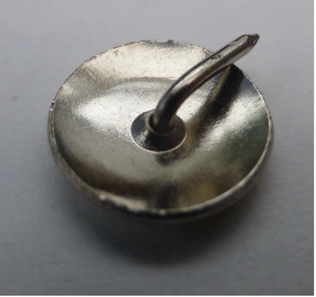
Much more slight damage, such as a bit of bending of the pin, might be less noticeable, but could lead to later trials being a little more likely to be heads than tails. In this case, the probability of heads is not a constant, but is gradually increasing, as the pin becomes increasingly bent. Then, the probability is conditional on whether it is an early or late trial.
A classic example contrasting independent and dependent trials is to imagine sweets in a bag - there could be \(1\) red sweet, \(2\) yellow sweets and \(3\) blue sweets. We assume the bag is opaque (we can’t see inside) and the sweets are identical in size and feel (and smell?). If someone takes a sweet from the bag at random, looks at it, replaces it in the bag, and takes another one, will these trials be dependent or independent?
If the bag is small, and we don’t shake it thoroughly in between trials, we could be more likely to get the same sweet again on the second draw, because it is near the top of the bag. Then, the probability of getting, say, the red sweet on the second draw would be greater if they had got a red sweet on the first draw than if they hadn’t. This means that the trials would not be independent. But if the bag is thoroughly shaken, we might expect the trials to be independent, and the probability of getting a red sweet would be \(\frac{1}{6}\) each time.
It is very important of course that the sweet is replaced after each trial – what we refer to as with replacement trials.
If the red sweet that is removed on the first trial is kept, and eaten, the probability of getting a red sweet on the second trial will obviously now be zero, since there are no more red sweets available. However, it is important to realise that the probability of getting each of the other sweets will also have changed, because there will be only \(5\) sweets remaining, and yet the total probability of drawing some sweet must still be \(1\).
This means that the probability of getting a yellow for instance, will have increased from \(\frac{2}{6}\) to \(\frac{2}{5}\), because although the number of yellow sweets hasn’t changed, the total number of sweets has dropped from \(6\) to \(5\). Because the red sweet is gone, the other two colours of sweet are both now more likely than they were on the first trial, because there are just fewer sweets to select from in total. This time we are doing without replacement trials. I generally think learners don’t spend enough time thinking about independent and dependent events and with- and without-replacement trials.
We are now thinking about combinations of events, and a key representation for this is the tree diagram, as shown in Figure 5.26 for two sweets being drawn at random, one after the other, with replacement. We use the notation \(R_{2}\), for example, to mean that a red sweet is drawn on the second draw.

For the with-replacement scenario, returning the sweet after each draw, the probabilities will be the same each time: always \(\frac{1}{6}\) for red, \(\frac{2}{6}\) for yellow and \(\frac{3}{6}\) for blue. It is often helpful to avoid cancelling down fractions when calculating probabilities, because then it is easier to see at a glance that
\[\frac{1}{6} + \frac{2}{6} + \frac{3}{6} = 1\]
than that
\[\frac{1}{6} + \frac{1}{3} + \frac{1}{2} = 1.\]
Because we are replacing the sweet after each trial, we can go on drawing out sweets for as long as we want, because the bag is returned to its original condition after each draw.
We can see that
\[P\left( R_{1} \right) = P\left( R_{2} \right) = \frac{1}{6}.\] \[P\left( Y_{1} \right) = P\left( Y_{2} \right) = \frac{2}{6}.\] \[P\left( B_{1} \right) = P\left( B_{2} \right) = \frac{3}{6}.\]
The subscripts here are not making any difference to the probabilities, and we could just write
\[P(R) = \frac{1}{6} \qquad P(Y) = \frac{2}{6} \qquad P(B) = \frac{3}{6} .\]
The probability \(P\left( R_{1} \cap R_{2} \right)\) of getting a red sweet followed by another red sweet will be
\[P\left( R_{1} \cap R_{2} \right) = P(R)\ P(R) = \frac{1}{6} \times \frac{1}{6} = \frac{1}{36} ,\]
because, in the long run, \(\frac{1}{6}\) of the first draws will give a red sweet, and \(\frac{1}{6}\) of the second draws will give a red sweet, so \(\frac{1}{6}\) of \(\frac{1}{6}\) of the first two draws will give two red sweets.
Similarly,
\[P\left( Y_{1} \cap Y_{2} \right) = P(Y)\ P(Y) = \frac{2}{6} \times \frac{2}{6} = \frac{4}{36}\]
\[P\left( B_{1} \cap B_{2} \right) = P(B)\ P(B) = \frac{3}{6} \times \frac{3}{6} = \frac{9}{36}.\]
These are compound probabilities – the probabilities of a combination of events, as indicated by the intersection symbol \(\cap\).
These events are independent, but, whatever the scenario, we always multiply the probabilities when we travel along consecutive branches of a tree diagram.
Learners are often confused by this, because they think you can only multiply probabilities when the events are independent, but we can see that it works the same way when we eat the sweets and have dependent events.
Now, although \(P\left( R_{1} \right) = \frac{1}{6},\) as before, this time the probability of \(R_{2}\) depends on what has happened on the first draw - it becomes a conditional probability. There are three different “\(P\left( R_{2} \right)\)”s.
We write \(P\left( R_{2} \middle| R_{1} \right)\) to mean the probability of getting red on the second draw, given that we got red on the first draw. This probability must be zero, because there is only one red sweet, so if a red sweet appears on the first draw, then it is eaten, and will never appear again.
Thinking in this kind of way, we can compute the \(9\) conditional probabilities below:
\[ \begin{array}{ccc} \displaystyle P\left( R_{2} \middle| R_{1} \right) = \frac{0}{5} & \displaystyle P\left( R_{2} \middle| Y_{1} \right) = \frac{1}{5} & \displaystyle P\left( R_{2} \middle| B_{1} \right) = \frac{1}{5} \cr \displaystyle P\left( Y_{2} \middle| R_{1} \right) = \frac{2}{5} & \displaystyle P\left( Y_{2} \middle| Y_{1} \right) = \frac{1}{5} & \displaystyle P\left( Y_{2} \middle| B_{1} \right) = \frac{2}{5} \cr \displaystyle P\left( B_{2} \middle| R_{1} \right) = \frac{3}{5} & \displaystyle P\left( B_{2} \middle| Y_{1} \right) = \frac{3}{5} & \displaystyle P\left( B_{2} \middle| B_{1} \right) = \frac{2}{5} \end{array} \]
To find the compound probabilities, these are the multipliers (Chapter 1) we need to use.
For example, to find \(P(Y_{1}{\cap R}_{2})\) we first draw a yellow, with probability \(P\left( Y_{1} \right) = \frac{2}{6},\) and then, given that the first draw was yellow, we draw a red, with probability \(P\left( R_{2} \middle| Y_{1} \right) = \frac{1}{5}\). In the long run, on \(\frac{2}{6}\) of the first draws, we will get a yellow, and, given this has already happened, on \(\frac{1}{5}\) of the second draws we will get a red. So, on \(\frac{2}{6}\) of \(\frac{1}{5}\) of the first two draws, we will get a yellow followed by a red.
So, \[P\left( Y_{1}{\cap R}_{2} \right) = P\left( Y_{1} \right)\ P\left( R_{2} \middle| Y_{1} \right) = \frac{2}{6} \times \frac{1}{5} = \frac{2}{30}.\]
In general, for any two events \(A\) and \(B\),
\[P(A \cap B) = P(A)\ P\left( B \middle| A \right).\]
In terms of multipliers,
\[ \begin{matrix} P(A) & \fixedarrow{$\times \ P\left( B \middle| A \right)$} & P(A \cap B) . \\ \end{matrix} \]
For \(A\) and \(B\) both to happen, \(A\) must happen, and then \(B\) must happen, given that \(A\) has already happened.
Learners are sometimes told ‘You only multiply probabilities when the events are independent’, but this can be confusing. Here the events \(Y_{1}\) and \(R_{2}\) are dependent, but we multiply, just as with independent events - we just have to make sure the second probability is conditional on the first. As in the with-replacement example, we multiply as we flow along the branches of the tree, because each fraction we obtain on a branch applies to all of the probability that ‘flows into’ that branch.
The only change to the tree diagram in Figure 5.27 for dependent events is that the \(R_{2}\), \(Y_{2}\) and \(B_{2}\) events in the second stage have probabilities that depend on which branch of the first stage (\(R_{1}\), \(Y_{1}\) and \(B_{1}\)) they follow, so they become conditional events.

We can calculate the \(9\) compound probabilities in Figure 5.27:
\[ \begin{array}{ccc} \displaystyle P(R_{1} \cap R_{2}) = \frac{1}{6} \times \frac{0}{5} = \frac{0}{30} & \displaystyle P(Y_{1} \cap R_{2}) = \frac{2}{6} \times \frac{1}{5} = \frac{2}{30} & \displaystyle P(B_{1} \cap R_{2}) = \frac{3}{6} \times \frac{1}{5} = \frac{3}{30} \cr \displaystyle P(R_{1} \cap Y_{2}) = \frac{1}{6} \times \frac{2}{5} = \frac{2}{30} & \displaystyle P(Y_{1} \cap Y_{2}) = \frac{2}{6} \times \frac{1}{5} = \frac{2}{30} & \displaystyle P(B_{1} \cap Y_{2}) = \frac{3}{6} \times \frac{2}{5} = \frac{6}{30} \cr \displaystyle P(R_{1} \cap B_{2}) = \frac{1}{6} \times \frac{3}{5} = \frac{3}{30} & \displaystyle P(Y_{1} \cap B_{2}) = \frac{2}{6} \times \frac{3}{5} = \frac{6}{30} & \displaystyle P(B_{1} \cap B_{2}) = \frac{3}{6} \times \frac{2}{5} = \frac{6}{30} \end{array} \]
These \(9\) compound events must sum to \(1\), because they are mutually exclusive, and there are no other possible outcomes from two draws. As we progress through successive events in a tree diagram, the outcomes extending from any single node are mutually exclusive and exhaustive, representing a complete sample space, so their probabilities must sum to \(1\).
In the with-replacement scenario, with the sweets going back into the bag, the probabilities are independent, and constant. For example, \(P\left( Y_{2} \middle| R_{1} \right) = P\left( Y_{2} \middle| Y_{1} \right) = P\left( Y_{2} \middle| B_{1} \right)\), and we can write all three as just \(P(Y_{2})\), or just \(P(Y)\).
In the without-replacement scenario, we can now see that if we wanted \(P\left( Y_{2} \right)\), say, meaning the total probability of getting yellow on the second draw, we would need to add up the three different, mutually exclusive ways in which this can happen:
\[P\left( Y_{2} \right) = P\left( R_{1}{\cap Y}_{2} \right) + P\left( Y_{1}{\cap Y}_{2} \right) + P\left( B_{1}{\cap Y}_{2} \right)\]
\[= \frac{2}{30} + \frac{2}{30} + \frac{6}{30} = \frac{10}{30}.\]
When we are selecting with replacement, we can continue removing sweets for as long as we wish, since they are going back in each time. So, the corresponding tree diagram can continue indefinitely. But in the without-replacement condition, there are only \(6\) sweets in total, so the tree diagram will have \(6\) levels before it terminates. For the final level, there will be only one sweet remaining, so the conditional probability will necessarily be \(1\).
5.6.3.2 Bayes’ Theorem
In general, if events \(A\) and \(B\) are independent, then
\[P\left( A \middle| B \right) = P\left( A \middle| B' \right) = P(A).\]
Event \(A\) doesn’t care about whether event \(B\) happened, or didn’t happen. Their probabilities are completely unconnected.
We have seen that the probability that \(A\) and \(B\) both happen will always be the probability that \(A\) happens, multiplied by the probability that \(B\) happens, given that \(A\) has already happened:
\[P(A \cap B) = P(A)\ P\left( B \middle| A \right).\]
Equivalently, we could say that the probability that \(A\) and \(B\) both happen will be the probability that \(B\) happens, multiplied by the probability that \(A\) happens, given that \(B\) has already happened:
\[P(A \cap B) = P(B)\ P\left( A \middle| B \right).\]
This works because \(A \cap B\) and \(B \cap A\) represent the same thing. When we say ‘already’ we don’t necessarily mean this chronologically - we are not saying that either \(A\) or \(B\) has to have happened first. We are saying we ‘already’ know and take account of the fact that it happens, regardless of the actual timing.
The only difference if \(A\) and \(B\) are independent events is that \(P\left( B \middle| A \right)\) can be simplified to \(P(B)\), which gives us the formula
\[P(A \cap B) = P(A)\ P(B).\]
We can link this back to the Venn diagram in Figure 5.17.
We saw in Section 5.6.1 that for any two events \(A\) and \(B\),
\[P(A \cup B) = P(A) + P(B) - P(A \cap B).\]
This formula is always true, but under the constraint that \(A\) and \(B\) are independent, we can replace \(P(A \cap B)\) with \(P(A)\ P(B)\), to obtain
\[P(A \cup B) = P(A) + P(B) - P(A)P(B).\]
Learners often confuse mutually exclusive events with independent events, or, at least, do not fully appreciate how they are similar and distinct. The following task can help with this:41
Invent possible values for \(P(A)\), \(P(B)\), \(P(A \cup B)\) and \(P(A \cap B)\) so that events \(A\) and \(B\) are ..
1. … mutually exclusive
2. …independent.
Can events \(A\) and \(B\) be both mutually exclusive and independent?
Why / why not?
There are many tasks that can help learners think about these relationships.
For example:42
One child had a cold, and when they got better their sibling got a cold.
The parent said, “When you have two children, there’s twice as much probability that one of them will be ill”.
What is wrong with this statement?
It cannot be true that the probability doubles.
We can see that by supposing that the probability of one child getting ill is \(p\).
If \(p > 0.5\), then doubling it would lead to an impossible probability greater than \(1\).
Even if \(p < 0.5\), with enough children, you would end up with a probability greater than \(1\).
With \(n\) children, \(np > 1\) as soon as \(n > \frac{1}{p}\), so it cannot be right that probabilities add up in this way. The incorrect reasoning is to double-count the instances when more than one child is simultaneously ill.
A task for learners confident with algebraic inequalities is the following:43
For two independent events \(A\) and \(B\), how can we be sure that the formula \[P(A \cup B) = P(A) + P(B) - P(A)P(B)\] will not produce values for \(P(A \cup B)\) that are outside the \(0\) to \(1\) interval?
Bayes’ Theorem allows us to invert probabilities, and convert from \(P\left( B \middle| A \right)\) to \(P\left( A \middle| B \right)\).
We can think of getting to the compound event \(A \cap B\) in two different orders, as shown by the tree diagrams in Figure 5.28.

Because \(P(A \cap B)=P(B \cap A)\), it follows that
\[P\left( B \middle| A \right)\ P(A) = P\left( A \middle| B \right)\ P(B) ,\]
because both of them are equal to \(P(A \cap B)=P(B \cap A)\).
This means that if we know, say, \(P\left( A \middle| B \right),\) \(P(A)\) and \(P(B)\), we can work out \(P\left( B \middle| A \right)\), the inverse probability of \(P\left( A \middle| B \right)\).
5.6.3.3 The base-rate fallacy
The base-rate fallacy is a very common source of confusion that has real-life consequences, and even people who need to use this in their job often get it wrong! It requires some hard thinking to make sense of, but no difficult theory or algebra, so even quite young learners can be exposed to the idea.
Suppose there is an infection going around, and to keep things simple let’s suppose that everyone is either infected or uninfected. There are no awkward inconclusive cases or people waiting for test results, and so on.
Some people are in hospital and some people aren’t, and let’s suppose that is also a clear-cut binary - there are no complicated cases of people about to be discharged or waiting in a corridor for a bed.
Let’s also imagine that some but not all of the infected people are in hospital, and some but not all of the uninfected people are also in hospital.
A common, convenient way to represent data like this is in a two-way table, also called a contingency table, as shown below.
\[ \begin{array}{l|ccc} & \text{Infected } (I) & \text{Uninfected } (I') & \text{Total} \\ \hline \text{In Hospital } (H) & 38 & 62 & 100 \\ \text{Not in Hospital } (H') & 162 & 738 & 900 \\ \hline \text{Total} & 200 & 800 & 1000 \end{array} \]
The cells in a contingency table contain the frequencies (counts of the number of people, so they have to be non-negative integers).
We have two discrete random variables: infection status (the columns) and hospitalisation (the rows).
The variables are discrete, because they take a fixed number of values (called the levels of the variables). Infection status can be ‘infected’ (\(I\)) or ‘uninfected’ (\(I'\)); hospitalisation can be ‘in hospital’ (\(H\)) or ‘not in hospital’ (\(H'\)). As before, we are using the \('\) symbol to indicate the complement of an event.
Someone might look at these data and say, “There are more infected people not in hospital than in hospital. That means I’m more likely to meet an infected person in the street than in the hospital!”
What do you think about this statement?
It is true that there are more infected people not in hospital than in hospital, as shown by the first column in the table above. But there are also (a lot) more uninfected people not in hospital than in hospital, as shown by the second column, because there are just a lot more people not in hospital than in hospital. Comparing the raw numbers does not give you the full picture; we need to think about these numbers as fractions with different denominators.
A person randomly selected from those in hospital is much more likely to be infected than a person randomly selected off the street, which is presumably what really matters if you are worried about becoming infected.
Learners will be able to make sense of this by comparing the probabilities:
\[P\left( \text{infected if in hospital} \right) = \frac{38}{100} = 0.38\]
\[P\left( \text{infected if }\text{not}\text{ in hospital} \right) = \frac{162}{900} = 0.18.\]
The first probability is more than twice the second.
Both of these are probabilities that are someone is infected, but they are conditional on different things. The probability of being infected is conditional on whether you are in hospital or not, because these two numbers are different.
We often write it as \[P\left( I \middle| H \right) = 0.38 \qquad \text{ and } \qquad P\left( I \middle| H' \right) = 0.18.\]
Conditional probabilities are just about having different denominators - changing our perspective on what our probability is ‘out of’. Base-rate fallacy refers to neglecting to think about what the denominator is, and confusing something like \(P\left( I \middle| H \right)\) with something like \(P\left( I \middle| H' \right)\) - or assuming that they must be equal.
To work out \(P\left( I \middle| H \right)\), we need all the people who are infected and in hospital, as a fraction of all the people who are in hospital, whereas to work out \(P\left( I \middle| H' \right)\) we need all the people who are infected and not in hospital, as a fraction of all the people who are not in hospital.
\[ \begin{array}{cc} \displaystyle P\left( I \middle| H \right) = \frac{P(I \cap H)}{P(H)} & \qquad \displaystyle P\left( I \middle| H' \right) = \frac{P(I \cap H')}{P(H')} \end{array} \]
From the information in the table below, work out the eight conditional probabilities listed. \[
\begin{array}{l|ccc}
& \text{Infected } (I) & \text{Uninfected } (I') & \text{Total} \\
\hline
\text{In Hospital } (H) & 38 & 62 & 100 \\
\text{Not in Hospital } (H') & 162 & 738 & 900 \\
\hline
\text{Total} & 200 & 800 & 1000
\end{array}
\]
\[
\begin{array}{cccc}
P\left( I \middle| H \right) & \qquad P\left( I \middle| H' \right) & \qquad P\left( H \middle| I \right) & \qquad P\left( H \middle| I' \right) \\[1.5ex]
P\left( I' \middle| H \right) & \qquad P\left( I' \middle| H' \right) & \qquad P\left( H' \middle| I \right) & \qquad P\left( H' \middle| I' \right)
\end{array}
\]
What relationships are there among them? Why?
Each vertical pair of complementary events have probabilities that must sum to \(1\).
The denominators are the same, and the numerators are the probabilities of complementary events.
As we have seen, Bayes’ Theorem allows us to invert probabilities, and convert from \(P\left( I \middle| H \right)\) to \(P\left( H \middle| I \right)\).
By writing
\[ \begin{array}{cc} \displaystyle P\left( I \middle| H \right) = \frac{P(I \cap H)}{P(H)} & \qquad \text{and} \qquad \displaystyle P\left( H \middle| I \right) = \frac{P(H \cap I)}{P(I)} , \end{array} \] we can see that the numerators are equal; Bayes’ Theorem is just about switching denominators.
It follows that
\[P\left( I \middle| H \right)P(H) = P\left( H \middle| I \right)P(I) ,\]
which means that if we know, say, \(P\left( I \middle| H \right)\), \(P(H)\) and \(P(I)\), we can work out \(P\left( H \middle| I \right)\), the inverse probability, as we saw in Section 5.6.3.2.
The classic example of base-rate fallacy is with medical tests.
Let’s take the same \(1000\) people, but instead of focusing on whether they are in hospital or not, we give each person a test for the illness. We will again assume that all tests give either a positive (\(P\)) or negative (\(P'\)) result, and the frequencies are given in the table below. ‘Positive’ indicates they could have the illness, but further tests would be needed to confirm this.
\[ \require{colortbl} \begin{array}{l|ccc} & \text{Infected } (I) & \text{Uninfected } (I') & \text{Total} \\ \hline \text{Test positive } (P) & 192 & \cellcolor{red} 48 & 240 \\ \text{Test negative } (P') & \cellcolor{yellow} 8 & 752 & 760 \\ \hline \text{Total} & 200 & 800 & 1000 \end{array} \]
No test is perfect, and every test will give some false results.
A false positive means that the person tests positive when they don’t have the disease (shaded red in the table). It is a ‘false alarm’, indicating that something is wrong when it isn’t.
We can work out the probability of this using the numbers in the table:
\[P\left( P \middle| I' \right) = \frac{48}{800} = 0.06 ,\]
which is a \(6\%\) false positive rate. This sounds very low, so the test seems like a good test.
A false negative means that the person tests negative even though they do have the disease (shaded yellow in the table). Our test is failing to alert us when it should.
We can also work out the probability of this using the numbers in the table:
\[P\left( P' \middle| I \right) = \frac{8}{200} = 0.04 ,\]
which is a \(4\%\) false negative rate. Again, this sounds low and encourages us to believe the test is pretty good.
Now for the probability that the patient would actually care about, “If I test positive, what is the probability I have the infection?”
Given the low false positive and false negative rates, we would hope that this percentage would be very high.
When we calculate, we obtain \[P\left( I \middle| P \right) = \frac{192}{240} = 0.8 ,\] which is an \(80\%\) probability. This is high, but perhaps not as high as you might have expected. People tend to estimate a percentage over \(90\%\) for this, given the false positive and false negative percentages both being less than \(10\%\).
However, the thing to notice is that this crucial probability, \(P\left( I \middle| P \right)\), will drop much lower than \(80\%\) if the disease is relatively rare; i.e. if \(P(I)\) decreases.
Here, \[P(I) = \frac{200}{1000} = 0.2.\]
Let’s see what would happen if the disease were \(5\) times less prevalent, with \(P(I) = 0.04\) instead.
The table below shows the situation for a data set of \(10,000\) people.
\[ \begin{array}{l|ccc} & \text{Infected } (I) & \text{Uninfected } (I') & \text{Total} \\ \hline \text{Test positive } (P) & 384 & 576 & 960 \\ \text{Test negative } (P') & 16 & 9024 & 9040 \\ \hline \text{Total} & 400 & 9600 & 10{,}000 \end{array} \]
This time, the prevalence of the disease is much lower: \[P(I) = \frac{400}{10,000} = 0.04.\]
Only \(4\%\) of people have this disease.
Let’s check the false positive rate: \[P\left( P \middle| I' \right) = \frac{576}{9600} = 0.06 ,\] which is the same as before.
We can also check the false negative rate: \[P\left( P' \middle| I \right) = \frac{16}{400} = 0.04 ,\] which is also the same as before. In this sense, the test is equally reliable, and the only thing that has changed is that we are now dealing with a rarer disease.
Now, as before, we can calculate the probability that someone with a positive test result actually has the disease: \[P\left( I \middle| P \right) = \frac{384}{960} = 0.4 ,\] which is a \(40\%\) probability!
This is half the probability we had for the previous, more prevalent disease. Indeed, the probability has now dropped below \(50\%\); if you test positive for the disease, you probably don’t have it, which sounds counterintuitive! (Your doctor could say, “Good news - you just tested positive, which means you probably don’t have the disease!”)
What is happening now that the disease is rare is that there are lots of people who don’t have the disease, and so even with a low false positive rate, there will still be a lot of false positives. There are \(576\) false positives in the table above, which is more than the number of true positives (\(384\)). This means that if you get a positive test result, it is more likely to be a false positive than a true one.
However, you are still much more likely to have the disease if you test positive than if you test negative.
If you test negative, the probability you are infected is
\[P\left( I \middle| P' \right) = \frac{16}{9040} = 0.002, \text{ correct to 3 decimal places}.\]
Compared with this probability (less than \(0.2\%\)), a probability of \(40\%\) is huge, so in this sense a positive test result is certainly bad news, even though you are still less likely to have the disease than not.
A test may not be very useful when dealing with a rare disease, even if the false positive and false negative rates are low. This kind of situation confuses even medical professionals who are trying to interpret a positive test result for a patient, and is something everyone should understand.
5.6.4 Coins
When throwing two ordinary coins, learners may think that there are three equally-likely outcomes:
\[\text{both heads} \qquad \qquad \text{both tails} \qquad \qquad \text{one head and one tail.}\]
However, if they do some experiments, they will find that getting two heads happens about one-quarter of the time, not one-third. Although these three possibilities are mutually exclusive and exhaustive, they are not equally likely, because there are twice as many ways to get one head and one tail then there are to get two heads or two tails.44
The possibility space contains four equally-likely outcomes, and this can be easier to see if the two coins have different denominations or colours, as in Figure 5.29.

It is very valuable for learners to contrast the different benefits and drawbacks of tree diagrams, two-way tables and Venn diagrams for representing probabilities.45 We can represent the two coin throws in a tree diagram, as in Figure 5.30, and see the four equally-likely possibilities on the right-hand side.

5.6.5 Dice
Now let’s consider combinations of events with ordinary dice.
Twelve horses are numbered from \(1\) to \(12\).
Two ordinary dice are rolled repeatedly.
The total score each time determines which number horse moves forward \(1\) place.
The first horse to move \(10\) places to the finishing line wins.

How likely is each horse to win the race?
The first thing learners may realise is that Horse \(1\) will never leave the starting gate, because it is not possible to obtain a score of \(1\) by summing the numbers on two dice.
However, all the other \(11\) numbers can be obtained, although they are not equally likely. Learners are often surprised by this, even if they are experienced in playing board games such as Monopoly, in which a sense of how likely different totals are to appear gives a definite advantage.
Figure 5.31 shows a tree diagram for the possible outcomes when throwing two ordinary dice and adding their scores.

We can see that there are more different ways of making \(7\) than any other total, so \(7\) is the most likely outcome. It makes sense to predict a win for Horse \(7\) over any other horse, and if we play the horse race game enough times, Horse \(7\) will win most often.
We can also represent the situation in a possibility space table, as shown in Figure 5.32, where I have coloured one die white and the other black (Figure 5.33).


The probabilities range from \(\frac{1}{36}\) for a total of \(2\), to \(\frac{6}{36}\) for a total of \(7\), and then back down to \(\frac{1}{36}\) for a total of \(12\). The linear nature of the graph of probability against total score can be surprising to learners, as they might instead expect a curve.46
Learners sometimes assume that the probability of Horse \(7\) winning the race is \(\frac{6}{36}\), but this is just the probability of getting a total of \(7\) on any single throw of the dice.
The probability that Horse \(7\) will win depends on the number of ‘steps’ from start to finish (\(10\) steps in TASK 5.34).
The probability of Horse \(7\) winning increases as the number of steps increases, because it heightens Horse \(7\)’s advantage. For \(10\) steps, the probability that Horse \(7\) will win is difficult to calculate, but turns out to be \(0.415\), correct to \(3\) significant figures, which is much more than \(\frac{6}{36}\).47 With \(17\) or more steps to the finish, the probability of Horse \(7\) winning becomes greater than \(50\%\).
It is easy for learners to pose different dice-related tasks, such as this one:48
Throw three ordinary dice together.
How likely is it to get three consecutive numbers, such as \(3\), \(4\) and \(5\)?
Sometimes, analysis will be very complicated, and this can be an opportunity to highlight the practical value of simulations, both with real dice and using computers to model outcomes using pseudo-random number generators.
Similar tasks can be invented with spinners, which are easier to modify for different probabilities.49
5.7 What does modelling get us?
Understanding modelling gives learners not just the skill but the disposition to make and interpret mathematical models to solve problems and make sense in a wide range of situations that are not overtly mathematical. Not only will learners be able to estimate when asked to, but they will develop a habit of estimating before calculating, seeing that as normal behaviour. Anticipating the answer to a calculation puts learners in a strong position to sense-check what they are doing and ensure that their solutions are reasonable and useful.
In this section, I present a wide range of different tasks that exemplify a range of situations learners could handle.
5.7.1 Doughnuts
This is a rich task, sometimes known as the Frobenius coin problem.50
Identical doughnuts are sold in small bags of \(4\) or large bags of \(7\).
Can you buy exactly \(15\) doughnuts? Why / why not?
What numbers of doughnuts are possible or impossible to buy?
Learners may think \(15\) is impossible because it is neither a multiple of \(4\) nor a multiple of \(7\). However, with more thought they will realise that two small bags plus a large bag will give us \(2 \times 4 + 7 = 15\) doughnuts.
Clearly, any number smaller than \(4\) is impossible, as is any number between \(4\) and \(7\).
Learners could make a table of numbers and be systematic in finding out whether different numbers of doughnuts can or cannot be produced. Alternatively, they could combine \(4\)s and \(7\)s systematically, and see which numbers can be made. These two complementary approaches are illustrated in Figure 5.34, and both tend to arise when learners are presented with this task.

Beginning with the desired number of doughnuts forces learners to think about impossible doughnut numbers, whereas the two-way table approach raises the issue of whether some numbers of doughnuts might be made in more than one way.
Sometimes learners will use a number square and shade in numbers of doughnuts which can be made. If they can be encouraged to do this in four columns, as in Figure 5.35, this can be particularly helpful.

Often they will begin by just shading the multiples of \(4\) and \(7\), as in Figure 5.35(a). The multiples of \(4\) all appear in the right-hand column, and learners may notice the regular pattern in the shadings for the multiples of \(7\), shifting \(1\) column to the left and \(2\) rows up for each successive multiple. This reflects the fact that \(\frac{7}{4}=1\frac{3}{4}\) or \(7=3\text{ mod }4\).
Then they will realise that numbers like \(11\) (\(= 4 + 7\)) and \(15\) (\(= 2 \times 4 + 7\)) are also possible (Figure 5.35(b)).
A bigger realisation is that once any number in a column is shaded, we can immediately shade all the numbers above that number, because we can get to any of them by adding multiples of \(4\) to the shaded number.
Learners often realise this for the fourth column, which contains all the multiples of \(4\), but eventually realise that it is true for any column. In Figure 5.35(b), I have shaded \(14\), \(15\) and \(16\), which means that all higher numbers in columns \(2\), \(3\) and \(4\) must be possible.
We can’t make \(13\) or \(17\), but we can make \(21\), and so from then on upwards, all the numbers in column \(1\) will be possible, as indicated in Figure 5.35(c).
Once we get four consecutive numbers (\(18\), \(19\), \(20\), \(21\)), we can get every later number by adding \(4\)s to each of these. This reveals that \(17\) must be the highest impossible number,51 and provokes the question “Why \(17\) and not some other number?” It must depend on the bag sizes, \(4\) and \(7\), but how?
Will there always be a highest impossible number? No. If we had bag sizes of \(4\) and \(8\), for instance, then there wouldn’t be, as learners can see by thinking about the shadings.
For bag sizes of \(4\) and \(8\), we would only be able to shade numbers in the fourth column, so there would be no highest impossible number. Any number in columns \(1\), \(2\) or \(3\) would be impossible, no matter how high up we went. To have a highest impossible number, we need co-prime bag numbers.
Working in \(4\) columns is helpful here, because the smaller bag size is \(4\). Columns of \(7\) would also work, but be slightly more work. By writing the numbers in columns, we are effectively doing modular arithmetic (Chapter 4). The column number is the remainder on division by \(4\), with column \(4\) corresponding to a remainder of zero.
Learners can explore different possible bag sizes, including when there are more than two different bag sizes.
They will find that, for coprime bag sizes \(x\) and \(y\), the highest impossible number is \(xy - (x + y)\), which can also be written as \((x - 1)(y - 1) - 1\).
With \(x = 4\) and \(y = 7\), the highest impossible number is \(4 \times 7 - (4 + 7) = 17\), as we saw above.
Learners may also find that the total number of impossible numbers (of any size) is \(\frac{1}{2}(x - 1)(y - 1)\), which, for \(x = 4\) and \(y = 7\), gives \(\dfrac{3 \times 6}{2} = 9\), which matches the \(9\) unshaded squares in Figure 5.35(c).
We can prove our formulae by thinking about where the multiples of \(7\) land in our four columns.
Because \(4\) and \(7\) are coprime, each successive multiple of \(7\) comes in a different column.
In Figure 5.35, we see that \(7\) comes in column 3, \(14\) in column \(2\), \(21\) in column \(1\) and \(28\) in column \(4\). They will continue to cycle through the columns in this order. It follows that the last multiple of \(7\) to break into a new column will be the third one, because the fourth one has to be a multiple of \(4\), and we already have column \(4\) shaded out.
The number \(21\) was the last piece in the jigsaw, because it was the first number we hit in our final unshaded column.
The number \(21\) is \((4 - 1) \times 7\), but in general if we are working in \(x\) columns, the equivalent of \(21\) will be \((x - 1)y\), because it will be the final multiple of \(y\) before we reach \(xy\).
The highest impossible number must be \(x\) numbers back from this, and so will be \((x - 1)y - x\), which is equivalent to the expression \(xy - (x + y)\) we had earlier.
Of course, this expression has to be symmetrical in \(x\) and \(y\), which it is.
If we were working in \(7\) columns, rather than \(4\), but with the same bag sizes, the last piece in the jigsaw would be the \((7 - 1)\)th multiple of \(4\), or \((7 - 1) \times 4 = 24\). This is different from the \((4 - 1)\)th multiple of \(7\).
However, when we step back \(7\) from this number, to the number immediately underneath it in the \(7\)-column table, we will find \(24 - 7 = 17\), which is the same highest impossible number.
We can develop this task further.
A small bag of doughnuts costs \(£1\) and a large bag costs \(£1.50\).
If I need \(31\) doughnuts for a class of learners, what is the cheapest way to get the required number?
Learners will notice that the price per doughnut is less for the large bag, since \[\frac{1.5}{7} < \frac{1}{4},\] which is as we would expect.
This means that if we want to spend as little as possible, it is reasonable to try to buy as many large bags as we can.
However, although this is a sensible heuristic (strategy) to try, it is only guaranteed to be cheaper if we end up with exactly the required number of doughnuts, which will happen if the required number of doughnuts is a multiple of \(7\). If the required number of doughnuts is a multiple of \(4\), but not a multiple of \(7\) - for example, \(20\) doughnuts - then we may find that it is cheaper to buy more doughnuts than we need.
If we buy \(5\) bags of \(4\), we will get exactly the right number of doughnuts, but it will cost \(£5\), whereas if we buy \(3\) large bags, that will get us \(21\) doughnuts, and it will cost only \(3 \times 1.5\), or \(£4.50\). We save \(50\) pence by buying an extra doughnut! Learners may be very surprised that we are effectively being paid \(50\) pence to take away another doughnut.
It is useful to have a systematic way of finding out how we can buy a certain number of doughnuts, such as \(31\). Haphazard trial and effort is tedious and inefficient.
One strategy is to iteratively subtract multiples of the larger bag size, checking each time whether the result is a multiple of the smaller bag size. With bag sizes of \(4\) and \(7\), for example, we would subtract multiples of \(7\) from \(31\) until we hit a multiple of \(4\).
If we want to find all the possible solutions, rather than just one, we would continue subtracting \(7\)s until subtracting any more would take us below zero. Subtracting the larger bag size, rather than the smaller one, means fewer rows in our table, as shown below.
\[ \begin{array}{ccl} \hline x & 31 - 7x & \text{Is what's left a multiple of 4?} \\ \hline 0 & 31 & \phantom{\text{Is what's left a multiple of }}\text{No} \\ 1 & 24 & \text{Yes} \\ 2 & 17 & \phantom{\text{Is what's left a multiple of }}\text{No} \\ 3 & 10 & \phantom{\text{Is what's left a multiple of }}\text{No} \\ 4 & 3 & \phantom{\text{Is what's left a multiple of }}\text{No} \\ \hline \end{array} \]
From this table, we can see that, for \(x \geq 5\), where \(x\) is the number of large bags, the value of \(31 - 7x\) will be negative, so we stop the table at \(x = 4\).
Looking at the completed table, we can see that the only way to get exactly \(31\) doughnuts is to buy \(1\) large bag (\(x = 1\)), because that will leave \(24\) doughnuts, which is a multiple of \(4\), and so can be obtained from \(6\) small bags. This will cost \(1 \times 1.5 + 6 \times 1 = 7.5\), or \(£7.50\).
However, this is not the cheapest way to get at least \(31\) doughnuts.
To do that, it turns out to be better to buy \(32\) doughnuts. Learners might think this would involve buying \(8\) small bags, which would cost \(£8\), and be more expensive. However, if you buy \(4\) large bags and \(1\) small bag, you obtain \(32\) doughnuts, but it costs only \(4 \times 1.5 + 1 = 7\) or \(£7\), which is cheaper than buying exactly \(31\) doughnuts!
There are lots of assumptions here worth considering as part of building the model.
We assume the shop has unlimited numbers of both bag sizes. We assume that all the doughnuts are equally fresh and in the same condition. We assume that everyone is going to eat exactly one doughnut, whereas in practice someone might want more, or not like doughnuts at all. We assume that all \(31\) learners will be present that day. We have completely ignored the issue of different flavours and people’s preferences. Also, if you were going to buy such a large number of doughnuts, you might want to try to negotiate a deal with the shop to save even more money.
By varying the numbers of doughnuts in a bag, the number of different bag sizes, and the prices, there is a lot of potential for fruitful exploration.
Learners often begin this task by writing down an equation, such as \(7x + 4y = 31\), but then are unsure how to proceed. It is important to be clear what the letters are representing. Here, \(x\) is the number of large bags and \(y\) is the number of small bags. In an equation like \(c = 1.5x + y\), the letters \(x\) and \(y\) have the same meaning, but now \(c\) is the cost in pounds.
However, sometimes learners will write expressions such as \(x + 6y\) to mean ‘\(1\) large bag and \(6\) small bags’, and \(x\) and \(y\) could now be the number of doughnuts in each bag (\(7\) and \(4\)) or the price per bag in pounds (\(1.5\) and \(1\)), so it can become very muddling if learners do not define their letters clearly and ensure they are consistent.52
It is possible to invent and solve puzzles along these lines that seemingly do not have enough information.
For example, this task may look impossible to learners without additional information:
Small plates cost \(£3\) and large plates cost \(£7\).
I spent \(£32\) on plates.
How many plates did I buy?
Learners may set up an equation by letting the number of small plates be \(s\) and the number of large plates be \(l\).
Then
\[3s + 7l = 32.\]
This looks like simultaneous equations in two unknowns, but we have only one equation. Don’t we need another piece of information, such as: “I bought three times as many small plates as large plates”?
Then we could write
\[s = 3l ,\]
and solve these together to obtain \(l = 2\) and \(s = 6\). So, I bought \(2\) large plates and \(3\) small plates.
Converting “three times as many small plates as large plates” into \(s = 3l\) can be challenging.
The words “three times as many small plates” naturally makes learners want to write \(3s\), rather than \(3l\).53 Thinking about which there are more of (small plates) may help to get it the right way round.
Something similar is problematic when learners slip into ‘letter as object’ thinking.
For example, if there are \(d\) dogs and a total of \(l\) legs, then the number of legs will be \(4\) times the number of dogs, so \(l = 4d\), but learners may think this looks the wrong way round. They want to write \(d = 4l\), which they read as “dog equals four legs”, but this is thinking of the letter \(d\) as representing ‘a dog’, rather than the number of dogs.
To return to TASK 5.38, this extra information \(s = 3l\) is actually unnecessary.
Provided we know that the numbers of plates are positive integers, there is in fact only one solution to the single equation \(3s + 7l = 32\), and we do not need any further information.
The constraint that \(s\) and \(l\) must be positive integers makes this a Diophantine equation, and in this case this rules out any solution other than \(l = 2\) and \(s = 6\).
We can see this by using the same method as above, repeatedly subtracting \(7\)s from \(32\) and checking to see if we have a multiple of \(3\) leftover each time, as shown in the table below.
\[ \begin{array}{ccl} \hline l & 32 - 7l & \text{Is what's left a multiple of 3?} \\ \hline 0 & 32 & \phantom{\text{Is what's left a multiple of }}\text{No} \\ 1 & 25 & \phantom{\text{Is what's left a multiple of }}\text{No} \\ 2 & 18 & \text{Yes} \\ 3 & 11 & \phantom{\text{Is what's left a multiple of }}\text{No} \\ 4 & 4 & \phantom{\text{Is what's left a multiple of }}\text{No} \\ \hline \end{array} \]
Subtracting \(7l\) for \(l > 4\) will give negative values, so we can stop after \(l = 4\). This shows us that there is only one solution: \(l = 2\) and \(s = 6\).
By being systematic like this, we can be sure we can’t have missed any solutions. It is important that learners appreciate that this is a completely different strategy from searching haphazardly until you happen to find a solution, because in that case you wouldn’t know whether other solutions might exist as well. You wouldn’t know when it was safe to stop searching and conclude that no (other) solutions existed.
Learners can invent problems like this for each other, involving total amounts of money consisting of different-valued coins. When is there a unique solution and when is there more than one possibility?54
A provocative way to begin might be to pose the following question:
Why are there no \(£3\) coins?
What denominations of currency are most useful? Why?
Would a \(£15\) note be worth introducing? Why / why not?
I often find that learners have not previously thought about this. They may say, “Because \(3\) is an odd number”. But \(5\) is an odd number, and yet we have \(£5\) notes.
They might say, “Because not many things cost exactly \(£3\)”. Is that a good response?
5.7.2 Packing problems
Problems with a quick and easy - but wrong - answer can be great for stimulating learners to think more carefully about modelling. Packing problems often sound much easier than they are.
Here is a ‘trick’ task to begin with:
How many \(2 \times 3 \times 12\) cuboid packages can you fit inside a \(8 \times 9 \times 10\) cuboid box?
Learners may work out the volumes as \(2 \times 3 \times 12 = 72\) and \(8 \times 9 \times 10 = 720\) and conclude that, because \(72 \times 10 = 720\), they can fit \(10\) packages in the box.
However, the correct answer is zero, because the largest dimension of the package is \(12\), and this is greater than the largest dimension of the box that it is supposed to fit inside! Finding the multiplier of the volumes would be appropriate if we were dealing with a liquid, or a highly malleable solid, like modelling clay, but not for a rigid object. We are assuming that the packages cannot be deformed or broken up into pieces.
Actually, we are also assuming here that the packages have to lie flat inside the box. If they can go in at an angle, then we would need to use Pythagoras’ Theorem to decide whether one package might be able to fit inside the box or not, and in 3D this is quite a tricky problem.
There are important applications here when someone orders a delivery of something roughly cuboid-shaped (e.g. a large fridge) and wants to know whether it will fit inside a van or an elevator or whether they will be able to turn it around inside their hallway.
How many \(2 \times 2 \times 3\) cuboid packages can you fit inside a \(6 \times 6 \times 9\) cuboid box?
This time the answer certainly isn’t zero, because we can definitely fit at least one package inside the box. All three dimensions of the package are smaller than all three dimensions of the box, so it will go in any way round.
Let’s write the dimensions as \(\text{length} \times \text{width} \times \text{height}\). These are arbitrary words, and any of them can go in any direction, but we can decide to be consistent between the package and the box by putting the package in the box so that the package length is parallel to the box length, and so on.
If we do this in this example, we can see that the corresponding dimensions of the box are all \(3\) times those of the package, meaning that we can fit \(3\) packages in every row, \(3^{2}\) packages in every layer, and \(3^{3}\) packages in the entire box, with no spare room.
When the packages fit perfectly, we also get the correct answer by dividing the volumes: \[\frac{6 \times 6 \times 9\ }{2 \times 2 \times 3} = 3 \times 3 \times 3 = 27 .\] We can think of this as being because the quotient \[\frac{6 \times 6 \times 9\ }{2 \times 2 \times 3}\]
can be written as the product of the three separate integer quotients \[\frac{6}{2} \times \frac{6}{2} \times \frac{9}{3} .\]
How many \(3 \times 4 \times 5\) cuboid packages can you fit inside a \(5 \times 6 \times 8\) cuboid box?
Again, this time we can fill the entire box, because we can rotate the package until its \(\text{length} \times \text{width} \times \text{height}\) are \(5 \times 3 \times 4\), and then we will be able to fit in
\[\frac{5}{5} \times \frac{6}{3} \times \frac{8}{4} = 1 \times 2 \times 2 = 4.\]
In general, if we have a \(l \times w \times h\) package and a \(L \times W \times H\) box, we will be able to fit in the number of packages that is equal to whichever of these six quantities is the largest:
\[ \begin{array}{ccc} \displaystyle \left\lfloor \frac{L}{l} \right\rfloor \times \left\lfloor \frac{W}{w} \right\rfloor \times \left\lfloor \frac{H}{h} \right\rfloor & \hspace{3em} \displaystyle \left\lfloor \frac{L}{w} \right\rfloor \times \left\lfloor \frac{W}{h} \right\rfloor \times \left\lfloor \frac{H}{l} \right\rfloor & \hspace{3em} \displaystyle \left\lfloor \frac{L}{h} \right\rfloor \times \left\lfloor \frac{W}{l} \right\rfloor \times \left\lfloor \frac{H}{w} \right\rfloor \\[3ex] % \displaystyle \left\lfloor \frac{L}{l} \right\rfloor \times \left\lfloor \frac{W}{h} \right\rfloor \times \left\lfloor \frac{H}{w} \right\rfloor & \hspace{3em} \displaystyle \left\lfloor \frac{L}{w} \right\rfloor \times \left\lfloor \frac{W}{l} \right\rfloor \times \left\lfloor \frac{H}{h} \right\rfloor & \hspace{3em} \displaystyle \left\lfloor \frac{L}{h} \right\rfloor \times \left\lfloor \frac{W}{w} \right\rfloor \times \left\lfloor \frac{H}{l} \right\rfloor \end{array} \]
Here, the \(\left\lfloor \quad \right\rfloor\) notation is the floor function; i.e. the greatest integer less than or equal to the value (Chapter 4).
For example, if we are placing a length of \(4\) inside a length of \(11\), we can fit in two \(4\)s, but not \(3\), and so \[\left\lfloor \frac{11}{4} \right\rfloor = \left\lfloor 2.75 \right\rfloor = 2,\] rounding down, even though \(2.75\) is nearer to \(3\) than to \(2\).
Learners can invent quite challenging problems for each other based around these ideas. It can be quite surprising how many more packages can sometimes be fitted inside a box just by changing the orientations. One challenge is to invent problems in which there is a particularly dramatic difference, so the second best answer is considerably worse than the best answer.
So far, this is all just pure mathematics. Translating into real life is challenging, because of issues such as the thickness of the sides of the boxes. For example, if you had two identical \(5\ \text{m} \times 6\ \text{m} \times 8\ \text{m}\) wooden cuboid boxes, then neither would fit inside the other. One box would have to be a little smaller; or at least the walls would have to be a little elastic.
All of this also assumes that the dimensions are given with perfect accuracy.
If by ‘\(5\ \text{m} \times 6\ \text{m} \times 8\ \text{m}\)’ we mean only that these dimensions are correct to the nearest \(1\) m, then it might even be that a \(4.8\ \text{m} \times 5.7\ \text{m} \times 7.9\ \text{m}\) package would not fit inside a \(5\ \text{m} \times 6\ \text{m} \times 8\ \text{m}\) box, because any of the three dimensions of the package could be larger than the actual dimensions of the box! Taking account of this can lead to some challenging problems for learners to invent and solve.
A related problem is the following packing task:55
How much would it cost to send \(1000\) ordinary cubical dice through the post?
What do you think would be the cheapest way to pack them up?
A cube has the smallest surface area of any cuboid with the same volume, because it is closest to a sphere. So, the optimal solution will involve packing the dice \(10\) by \(10\) by \(10\).
If the dimensions of the cubes are \(1\) unit, then the volume will be \(1000\) cubic units and each square surface will have area of \(10 \times 10\), or \(100\) square units. Since there are six faces, the total surface area will be \(600\) square units.
We could take the dimensions of the dice as \(1\) cm, if they are very small dice. Then, depending on the shape of the wrapping paper, we would need at least \(600\) cm2 of paper - and realistically more.
Learners could look at how costs are calculated for sending parcels through the post and estimate the mass of their parcel. They could also consider the optimal cuboids for numbers of dice other than \(1000\), including where the number is not a cube number.
Real-life packing problems can be highly challenging. One way to make them more accessible is if the objects to be packed can be treated as identical, as in this case.
A nice task related to this is the following:56
Use an online maps app to find a local car park which has marked spaces for the cars.
It could be rectangular in shape or more irregular.
Imagine erasing all the white lines.
Can you redesign the layout to accommodate more cars?
Of course, you must ensure that the cars can get into and out of the spaces.
5.7.3 The tethered goat
Here is a well-known task that can be approached with an eye to modelling assumptions.57
A goat is tethered with a piece of rope to the outside corner of a shed in a field.
The dimensions of the shed are \(4\) m by \(3\) m.
How long should the rope be so the goat can graze \(50\) m2 of grass?
The grass in the field is unlikely to be of tennis-court quality, and so is going to be far from completely uniform. Given this, and that the area of \(50\) m2 is not specified very accurately, it would be sensible to make some quite coarse assumptions.
Assumptions could include:
The rope is inextensible and unbreakable.
The ground is flat and there are no obstacles in the field.
The field is large enough that the goat cannot reach the boundary.
The shed is rectangular, its sides are fixed and it is too tall for the rope to reach over.
The distance between the end of the rope and the goat’s mouth is negligible.
The goat moves out to every distance up to the maximum length of the rope.
The rope is indestructible and the goat cannot slip out of it.
Learners could continue stating assumptions, and perhaps order them according to (i) how necessary they are to simplify the problem, and (ii) how big a difference they are likely to make.
Learners are likely to begin by sketching different configurations.
For rope lengths \(r\) metres up to \(r = 3\), the area of grass accessed, \(A\) m2, will be three-quarters of a circle (Figure 5.36), so \[A = \frac{3\pi r^{2}}{4},\ \ 0 \leq r \leq 3.\]

By substituting \(r = 3\), we find that the maximum area obtained is \(21.2\) m2 (correct to \(1\) decimal place). This is less than \(50\) m2, so we need to think about what will happen if we extend the rope beyond \(3\) m.
Between \(3\) m and \(4\) m of rope, the rope will snag on the bottom right corner of the shed, and allow access to a little more grass. The area of grass is now three-quarters of a larger circle, plus one-quarter of a much smaller circle (Figure 5.37).

Learners often incorrectly draw a single arc, as in Figure 5.38.

This cannot be correct, because for the goat to reach point \(P\), the rope would have to pass through the shed, as shown by the dashed radius. In fact, it can reach around only as far as point \(Q\), which is a distance of \(4\) m from the centre of the circle, going around the shed.
Using the correct diagram, as shown in Figure 5.37, we have
\[A = \frac{3\pi r^{2}}{4} + \frac{\pi(r - 3)^{2}}{4},\ \ 3 \leq r \leq 4.\]
We can see that when \(r = 3\) this agrees with the previous formula, which is as we would require, since there is no sudden increase in area of grass available when the rope is let out just a tiny bit more.
Substituting \(r = 4\), we find that \(A = 38.5\), correct to \(1\) decimal place. So, the goat can access \(38.5\) m2 of grass - but this is still not enough.
If we let out more rope, we will gain another quarter of a circle at the top left of the shed. For example, with \(r = 5\) the situation will be as shown in Figure 5.39.

Now, \[A = \frac{3\pi r^{2}}{4} + \frac{\pi(r - 3)^{2}}{4} + \frac{\pi(r - 4)^{2}}{4},\ \ 4 \leq r \leq 7.\]
Learners may have to think hard to appreciate that this formula will be correct until the rope is \(7\) m long, but at that point the goat will be able to reach right around the shed by going either clockwise or anticlockwise. This is because \(7\) m is the semi-perimeter of the shed.
If we substitute \(r = 5\) into this formula, we obtain \(A = 62.8\), correct to \(1\) decimal place. This is quite a jump up in area.
Learners might use the squares on the sketches to estimate the areas. They might also draw a piecewise graph to show how \(A\) goes up as \(r\) increases.
We now know that the \(r\) value we are looking for must lie within the interval \(4 \leq r \leq 5\), because \(A(4) < 50 < A(5)\), and we have a smoothly-varying function in between.
We might decide that an answer of \(4.5\) m is near enough for practical purposes, given all the approximations we have made.
However, if we want to, we can obtain a more accurate answer by solving the equation
\[\frac{3\pi r^{2}}{4} + \frac{\pi(r - 3)^{2}}{4} + \frac{\pi(r - 4)^{2}}{4} = 50.\]
Simplifying,
\[3\pi r^{2} + \ \pi(r - 3)^{2} + \pi(r - 4)^{2} = 200\]
\[3r^{2} + r^{2} - 6r + 9 + r^{2} - 8r + 16 = \frac{200}{\pi}\]
\[5r^{2} - 14r + 25 - \frac{200}{\pi} = 0.\]
Using the quadratic formula,
\[r = \frac{14 \pm \sqrt{14^{2} - 4 \times 5 \times \left( 25 - \frac{200}{\pi} \right)}}{2 \times 5} ,\]
which gives \(r = 4.51\) or \(r = - 1.71\), correct to \(2\) decimal places.
The negative solution has no meaning, since a circle’s radius must be positive. So, we conclude that a \(4.51\) m rope would allow the goat to graze about \(50\) m2 of grass, and our estimate of \(4.5\) m above was actually quite accurate.
For \(r > 7\), the goat can reach the same parts of the grass by going in either direction around the shed, so we obtain a much more complicated and hard-to-calculate area, such as the one in Figure 5.40 for \(r = 8\).

However, from a modelling point of view, as \(r\) increases beyond \(7\), the shaded area approaches more closely a complete disc of radius \(r\), minus the shed, and \(\pi r^{2} - 4 \times 3\) becomes an increasingly good (over)-estimate for the area of grass the goat can access.
Putting additional buildings or other objects in the field makes finding the locus of positions the goat can reach more difficult, and this is true of the associated area as well.
5.7.4 The fastest route
This task tends to create a lot of energetic discussion:
A swimmer \(S\) in the sea shouts for a lifeguard \(L\) who is on the beach, as shown below.

The lifeguard could swim in a straight line from \(L\) to \(S\).
But, because the lifeguard can run faster than they can swim, should should they instead run along the beach some way and then swim to \(S\) from there?
If so, how far along the beach should they run before they start to swim?
Learners should realise that the answer will depend on the relative difference in speed between running and swimming.
If running were so much faster than swimming that we must maximise the amount of the journey which is running, then the fastest route would be to run almost \(4\) units to the right and then swim approximately \(3\) units out to the swimmer. But, in practice, there will be some trade-off between running and swimming that means they will be faster if they cease running a bit sooner than that (Figure 5.41).

Suppose the lifeguard’s running speed is \(3\) m/s and swimming speed is \(1\) m/s.
Let \(x\) metres be the distance \(LX\) in Figure 5.41, which the lifeguard runs before they begin swimming.
Let’s suppose the scale of Figure 5.41 is that each square has side length of \(10\) m.
Then, using Pythagoras’ Theorem, the time \(t\) seconds to get to the swimmer will be
\[t = \frac{x}{3} + \frac{\sqrt{30^{2} + (40 - x)^{2}}}{1}\]
\[= \frac{x}{3} + \sqrt{x^{2} - 80x + 2500}.\]
This is a messy function, but learners could use graph-drawing software to explore its properties; in particular, to find its minimum value and where it occurs (Figure 5.42).

Learners may be confused that time, \(t\), is plotted on the vertical axis, whereas often times is the independent variable, on the horizontal axis. Here, we are thinking of ‘time taken’ as being the dependent variable that depends on the lifeguard’s choice of where on the beach to commence swimming from.
The exact values for the minimum of the function are \(x = 40 - \frac{15}{2}\sqrt{2}\) and \(t = \frac{40}{3} + 20\sqrt{2}\), but learners may focus on obtaining approximate values from the graph: \(x = 29.39\) and \(t = 41.62\), both correct to \(2\) decimal places.
This means that the optimal position for the lifeguard to begin their swim is about \(29\) m from \(L\), and the entire route will take about \(42\) seconds.
Learners can compare this with swimming in a straight line from \(L\) to \(S\), which will take \(\frac{50}{1} = 50\) seconds, as we can also see from the \(t\)-intercept in Figure 5.42, and by substituting \(x = 0\) in the equation for \(t\).
The other comparison learners may make is with running \(40\) metres along the beach and then swimming \(30\) metres to \(S\), perpendicular to the beach.
This will take \[\frac{40}{3} + \frac{30}{1} = 43\frac{1}{3} \text{ seconds},\]
which is much shorter than the direct route but not quite as short as the shortest possible route.
Of course, there are a lot of assumptions in play here, such as that the lifeguard has constant running and swimming speeds, and does not tire over time, or find some parts of the beach or sea faster or slower to run or swim in than others. We also assume that the swimmer stays in one location and does not drift around.
This problem is analogous to what happens in the refraction of light. When a ray of light passes from a less dense medium, such as air, to a denser medium, such as glass, it changes its direction of travel, as if it were trying to get to its destination more quickly than nearby, neighbouring paths that it could have taken instead,58 and this is described by Snell’s Law.
Other problems concerning the shortest distance to a destination can also draw on Pythagoras’ Theorem.59
The following task is based on an application of the region-beta paradox:60
If I have to travel more than \(1\) mile, I cycle.
If I have to travel less than \(1\) mile, I walk.
Sketch a graph of what my journey times might look like for journeys of different total distances.
We can suppose that cycling speed \(v_{c}\) is greater than walking speed \(v_{w}\), and since journey time is inversely proportional to mean speed, when we plot journey time \(t\) hours against total distance \(d\) miles, we expect to obtain two straight lines through the origin but with different gradients.
The line for time if cycling, \(t_{c}\), will have gradient \(\dfrac{1}{v_{c}}\), and the line for time if walking, \(t_{w}\), will have larger gradient \(\dfrac{1}{v_{w}}\), because \(v_{c} > v_{w}\).
The gradient is larger for walking because it takes more time to cover the same distance.
For the same \(d\), the we have \(t_{c} < t_{w}\), because
\[t_{c} = \frac{d}{v_{c}} < \frac{d}{v_{w}} = t_{w}.\]
The two time graphs are shown in Figure 5.43(a), with the relevant portions indicated with a solid line in Figure 5.43(b).

We obtain a non-monotonic relationship, where increasing \(d\) beyond \(1\) initially leads to a decrease in \(t\).
The discontinuity at \(d = 1\) means that travelling a greater distance may be quicker. I might not have time to go \(0.9\) miles, but I might have time to go \(1.1\) miles! Learners may find this counterintuitive, but it should fit with their personal experience of travelling around by different modes of transport.
If we take mean walking speed as \(3\) mph and mean cycling speed as \(10\) mph, as in Figure 5.43, we can calculate the bounds of the so-called ‘region beta’, in which travelling further takes less time.
We need to find out when the cycling time becomes as great as the walking time is for \(1\) mile.
The walking time for \(1\) mile is \(\dfrac{1}{3}\) hour, or \(20\) min.
The distance we can cycle in \(20\) min is \(\dfrac{10}{3} = 3\dfrac{1}{3}\) miles.
So, ‘region beta’ is from \(1\) mile to \(3\dfrac{1}{3}\) miles.
For distances greater than \(3\frac{1}{3}\) miles, there are no shorter distances which take longer to get to, so we are no longer within ‘region beta’. The mathematics here is just straight-line graphs, but careful thought is needed to figure out all of this without getting confused!
5.7.5 Buying coffee
Sometimes, real-life situations require very minimal formal mathematics, but just a little bit of mathematical reasoning.
Here is an example in which inequalities turn out to be surprisingly powerful. This is a true story:61
In a coffee shop, someone brought coffees for their friends, saying, “No way! I ordered five but he only gave me four!”
One of the friends responded, “Are you sure? How much did you pay?”
The person who brought the coffees replied, “I don’t remember, but it was \(12\) pound something, and they were \(2\) pound something each”.
What can you deduce from this?
Learners will often think that they can’t deduce anything unless they know the exact prices of the coffees and how much exactly was paid. This is what the people in the coffee shop thought - they felt that they needed the exact prices - and a calculator. But actually a conclusion can be reached with no more information and with minimal calculation.
The person bringing the coffees is saying that
\[£2 < \text{ cost of one coffee } < £3,\]
which means that
\[£8 < \text{ cost of $4$ coffees } < £12,\]
and
\[£10 < \text{ cost of $5$ coffees } < £15.\]
Even if the coffees were not all the same price, we are told that they cost between \(£2\) and \(£3\).
Four coffees, therefore, cannot exceed \(£12\). So, if the total cost really was ‘\(12\) pound something’, then they must have bought more than four coffees, and so they are right that they are missing a coffee!
Learners could try to invent tasks like this one for each other, which can be solved with minimal calculation.
5.7.6 Recipes
Recipes provide a nice, real-life context for doing some non-trivial mathematics, when it comes to limiting amounts of ingredients.
Here is a recipe for making \(12\) pancakes:
\(100\) g plain flour
\(300\) ml milk
\(2\) large eggs
\(1\) tbsp vegetable oil
I check in my cupboards and I have this much of each ingredient:
\(500\) g flour
\(800\) ml milk
\(6\) eggs
What is the maximum number of pancakes I can make?
The key is to find the ingredient with the smallest multiplier (Chapter 1) from the recipe to the quantity I have in my cupboard. This will then be the limiting ingredient that will determine how much I can scale up the entire recipe.
We will assume I have plenty of vegetable oil and that my flour is plain and my eggs are ‘large’. We will also assume I want to make as many pancakes as I can.
The table below shows the relevant calculations.
\[ \require{colortbl} \begin{array}{ccccc} \hline \text{Ingredient} & \text{Recipe} & \text{Cupboard} & \text{Multiplier} & \text{Amount to use} \\ \hline \text{flour} & 100\text{ g} & 500\text{ g} & \displaystyle \frac{500}{100} = 5 & 2.6 \times 100 = 260\text{ g} \\[2ex] \cellcolor{#D3D3D3} \text{milk} & \cellcolor{#D3D3D3} 300\text{ ml} & \cellcolor{#D3D3D3} 780\text{ ml} & \cellcolor{#D3D3D3} \displaystyle \frac{780}{300} = 2.6 & \cellcolor{#D3D3D3} \begin{array}{c} 780\text{ ml} \\ \text{limiting ingredient} \end{array} \\[2ex] \text{eggs} & 2 & 6 & \displaystyle \frac{6}{2} = 3 & \begin{array}{c} 2.6 \times 2 = 5.2 \\ 5\text{ eggs} \end{array} \\[2ex] \hline \text{Number of pancakes} & 12 & & & \begin{array}{c} 2.6 \times 12 = 31.2 \\ \text{about } 30\text{ pancakes} \end{array} \\ \hline \end{array} \]
Milk has the smallest multiplier (\(2.6\)), so the quantity of milk in the cupboard is going to limit how many pancakes I can make. I cannot use all the flour or eggs I have available, because there isn’t enough milk to do so, so the amount of those ingredients that I will actually use will be determined by the milk multiplier (\(2.6\)).
It is important with these problems to ensure that the ingredient which is most limiting does not come first on the list, otherwise learners may get the right answer without appreciating that it was determined by the quantity of that ingredient.
5.7.7 Aspect ratios
Aspect ratios come up in many different situations.
The ratio of the height to the base of a rectangle is its aspect ratio. This may be relevant when doing a presentation, photocopying, watching television or seeing a movie at the cinema. If the aspect ratio of what you are looking at doesn’t match the aspect ratio of what you are watching it on, the picture will either be stretched and distorted or there will be empty areas around the edges of the image - or some of the picture will be missing.
A common example in many countries are the A-series paper sizes, such as A4 paper:
What is special about A-size paper?
What happens when you fold a sheet of A-size paper in half?
Why does this happen?
When you fold a piece of A4 paper in half ‘lengthways’, you get a sheet of A5 paper which has half the area but exactly the same ‘shape’. Its aspect ratio is the same, and this is very useful if you want to enlarge or reduce a sheet onto another sheet, for example when printing or using a photocopier. It is also useful if you want to fold an A3 sheet, say, to make the cover for an A4 booklet.
People sometimes think that A-size paper is \(1:2\), but it can’t be.
If you fold \(1:2\) paper in half, you get \(1:1\) paper, which would be square (Figure 5.44).

Because the area halves, people assume that that the multiplier between the edges must also be \(2\), but actually when the area scale factor is \(2\) the length scale factor must be \(\sqrt{2}\) (Chapter 3).
We can see this in Figure 5.45.

If the folded sheet, when turned \(90{^\circ}\), has the same shape as the original sheet, then
\[\frac{1}{x} = \frac{\frac{1}{2}x}{1}.\]
Rearranging, \[2 = x^{2} ,\]
and, since \(x\) has to be a positive ratio, \(x = \sqrt{2}\), a so-called Silver Rectangle.
A4 paper is actually \(210\) mm \(\times\) \(297\) mm, so the ratio is \(\displaystyle \frac{297}{210}\), which is \(1.414...\), which is very close to \(\sqrt{2}\). The reason that both dimensions are awkward numbers is that A0 paper is set to have an area of \(1\) m2, meaning that for A0 paper we have to scale up our \(1:\sqrt{2}\) dimensions so that the product (i.e. the area) is equal to \(1\).
We obtain \[\frac{1}{\sqrt[4]{2}}:\frac{\sqrt{2}}{\sqrt[4]{2}} = \frac{1}{\sqrt[4]{2}}:\frac{\sqrt[4]{2}}{1} ,\]
and so A0 paper has to have dimensions \(\displaystyle \frac{1000}{\sqrt[4]{2}}\) mm, which is \(841\) mm, by \(\displaystyle \frac{1000\sqrt[4]{2}}{1}\) mm, which is \(1189\) mm.
‘A\(n\)’ paper therefore has dimensions \(\displaystyle \frac{841}{{\sqrt{2}}^{n}}\) mm by \(\displaystyle \frac{1189}{{\sqrt{2}}^{n}}\) mm, and for \(n = 4\) this gives approximately \(210\) mm by \(297\) mm.
More simply, the area of ‘A\(n\)’ paper is just \(2^{- n}\) m2, so A4 paper is \(\displaystyle \frac{1}{16}\) m2.
Here is a related problem:
I take a rectangular sheet of paper.
I remove a square from one end of the paper to leave a rectangle that is the same shape as the original rectangle.
What shape is the original rectangle?
If the original rectangle has dimensions \(1:x\), then a similar approach to the one with A4 paper leads to
\[\frac{1}{x} = \frac{x - 1}{1}.\]
Rearranging,
\[x^{2} - x - 1 = 0 ,\]
and, since \(x\) has to be a positive ratio, \(\displaystyle x = \frac{1 + \sqrt{5}}{2}\), a so-called Golden Rectangle, with many interesting properties.62
5.7.8 Folding a sheet of paper
Someone claims that you cannot repeatedly fold a sheet of paper in half more than \(7\) times.
Is this true?
Learners can try it with an ordinary sheet of paper, and will probably manage only about \(6\)-\(7\) folds. The folded paper eventually becomes too thick to fold over again. But why should the limit be around \(7\) folds, rather than some other number?
To model this problem, we can take the thickness of the paper as \(t\) metres and the dimensions of the paper as \(d\) metres (we will suppose it is square).
Every time we fold the paper, we double the thickness, so after \(n\) folds the thickness will be \(2^{n}t\) metres. And every time we fold twice, we halve the dimensions \(d\), so after \(n\) folds the dimensions will be \(\displaystyle \frac{d}{2^{\tfrac{n}{2}}}\).
Once the thickness approaches the dimensions of the paper, it will no longer be possible to fold it further.
So, we expect the maximum possible \(n\) to be somewhere near to the solution to
\[2^{n}t = 2^{- \tfrac{n}{2}}d.\]
As we have seen, a sheet of A4 paper is \(210\) mm \(\times\) \(297\) mm, which we could take as having dimensions of about \(20\) cm. Learners will not be able to measure its thickness directly, but they could take a ream of A4 paper (\(500\) sheets) and measure the thickness of the entire pack (about \(5\) cm for typical paper thickness). From this, they can estimate the thickness of one sheet as being about \(\frac{5}{100}\) cm, or \(0.0005\) m.
With \(d\) as about \(0.2\), we want to find \(n\) that solves
\[2^{n} \times 0.0005 = 0.2 \times 2^{- \tfrac{n}{2}}.\]
Simplifying, we obtain
\[2^{\tfrac{3n}{2}} = 400.\]
If learners know about logarithms, they can solve this directly; otherwise, they can use trial and improvement, as they only need to try a few small positive integers for \(n\).
Using logarithms, \[\frac{3n}{2} = \log_{2}400\]
\[n = \frac{2}{3}\log_{2}400 = 5.8,\] correct to \(1\) decimal place.
This fits with my experience, as I find I can manage only \(6\) folds. However, if you use a very large sheet of very thin paper, it is possible to fold it a few more times than this.
If it were possible to repeatedly fold a sheet of paper in half as many times as desired, how many folds would it take for the folded stack to reach to the moon?
Although, as we have seen, we can’t fold repeatedly very many times, we could imagine tearing a sheet of paper in half, stacking the sheets, tearing the stack in half, and so on. Eventually we wouldn’t be strong enough to tear the entire stack in half, but we could do so in batches, so we could in principle end up with a very tall stack of torn sheets.
In practice, the area would become so tiny it would be impossible to continue halving - and of course the stack of sheets would be far too precarious to balance!
The moon is about \(384,400\) km away, so now, working in metres, we need
\[2^{n}t = 384,400,000 ,\]
where \(t = 0.0005\), which gives
\[2^{n} = 768,800,000,000.\]
It follows that
\[n = \log_{2}{768,800,000,000} = 39.5,\] correct to \(1\) decimal place.
So, just \(40\) folds would be enough to get to the moon! Powers of \(2\) get big very quickly indeed.
5.7.9 Football on the roof
Here is a task inspired by a real-life situation in school.
Some students have lost a football on the top of a flat roof.
They want to know whether the ball has rolled down behind the back of the building, and is therefore gone forever, or whether it might be worth climbing up to try to retrieve it.63
The students do not have access to any tall buildings nearby that they could use to get a good view of the roof.
They walk back as far from the roof as possible, but cannot see the ball on the roof.

But does that mean the ball has gone, or might it just not be visible from that position, even if it is still sitting on the roof?
“Can you see it?”
“No, but maybe if I could just go back a bit further I would see it.”
“No, if it was there, you’d be able to see it by now.”
“I’m not sure.”
Do some calculations to decide.
Using similar triangles allows us to decide whether it is worthwhile to fetch a chair to stand on, and whether a search of the roof is justified or a waste of time. A full solution is available.64
5.7.10 Freehand circles
Learners may enjoy thinking about what measurements would be needed to judge a freehand circle-drawing competition:65
One a whiteboard, draw the best freehand circle you can.
How can we judge fairly whose circle is the best?
An electronic whiteboard or tablet is useful here, as each learner can draw their circle - only one attempt allowed! - and sign their name beside it, and then each image can be saved and shared. Then all learners can be tasked with deciding on a method to determine who is the winner.
Learners often suggest choosing points on the drawn circle and measuring how far they are from ‘the centre’. However, deciding where the centre is for a not-very-circular circle is challenging.
Another strategy is to measure multiple ‘diameters’ and find their standard deviation, but it can also be tricky to decide where diameters lie without a clear notion of ‘centre’ that they should go through.
Another problem with this idea is that it is possible to draw curves of constant width which are not circles. For example, the Reuleaux triangle shown in Figure 5.46 consists of three equal circular arcs, and has the same width in every direction, but is clearly not a circle. You could roll it along a flat surface and its top would trace out a straight horizontal line. But is centre would wobble up and down as it rolls along.

All curves of constant width have a perimeter equal to \(\pi\) multiplied by their width (Barbier’s Theorem), so that is also not a useful way to test if something is circular.
Another approach is to draw accurately over the hand-drawn circle two other precise circles: (i) the smallest circle that will just enclose it (the circumscribed circle) and (ii) the largest circle that will just fit inside it (the inscribed circle), as shown in Figure 5.47.
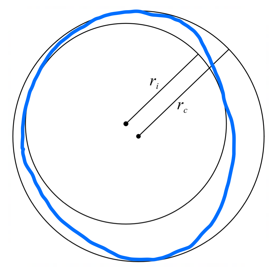
Roundness is defined as the ratio of the radius of the inscribed circle, \(r_{i}\), to the radius of the circumscribed circle, \(r_{c}\). A perfect circle will have a roundness of \(1\), because both of these circles will coincide exactly with the circle itself. But any non-circular shape will have an inscribed circle that is smaller than the circumscribed circle, and therefore a roundness less than \(1\). The circle in Figure 5.47 has a roundness of \(0.8\).
5.7.11 Survival tasks
The broadcaster and naturalist David Attenborough has described the challenges associated with his many treks into remote areas; in particular, the challenge of taking sufficient food with you.
He has stated:
“If one person who is not carrying food is accompanied by two others carrying full loads of provisions, the three of them will have enough food to last a fortnight. If a march lasts any longer than that, the number of food carriers needed starts to escalate very rapidly indeed and eventually becomes impossible to meet.”66
What mathematical sense can you make of this?
Learners might be surprised at this – they might assume that to last twice as long you would just need twice as many people carrying food. The problem with this is that the more people you bring with you, the more food they need too!
This task does not require much technical mathematical skill with algebra, but does require careful reasoning.
We could assume that everyone (carriers of food and non-carriers) all consume food at the same rate, and that all carriers carry the same amount of food.
Attenborough describes \(2\) carriers and \(3\) eaters having enough food to last \(14\) days. If, instead, everyone helped carry, we would have \(3\) carriers (and still \(3\) eaters), so there would be half as much food again for the same number of eaters, meaning that we would predict that they would be able to survive for half as long again, or \(21\) days.
This means that one person on their own, as a single eater and carrier, would also be able to last for \(21\) days.
It follows that \[\text{survival time }\left( \text{days} \right) = 21 \times\frac{ \text{number of carriers}}{\text{number of eaters}}.\]
Learners can explore this equation with \(n\) people, one of whom does not carry food.
A graph of number of carriers needed against survival time reveals the sharp increase beyond \(14\) days that Attenborough refers to.67
Based on these assumptions, there is an absolute upper limit of \(21\) days, because even if everyone carries and eats their own food, no one can carry more than is needed for \(21\) days.68 So, the graph has a vertical asymptote at \(21\) days.
Here is another task related to surviving in the wilderness:
A camel has to carry \(1800\) bananas across a \(600\)-mile desert.
The maximum number of bananas the camel can carry at any one time is \(600\).
The camel eats \(1\) banana for every mile it travels.
What is the maximum number of bananas that can reach the other side of the desert?
There are clearly some unrealistic aspects of this problem, such as the precise regularity with which the camel eats the bananas, as well as its ability to strategise! We assume all the bananas are of equal size and equally nutritious. We assume the terrain is uniform. We assume that none of the bananas are taken by any other animal, and so on.
Suppose the camel begins with \(b\) bananas and wants to transfer as many as possible across a distance of \(x\) miles.
If \(x \leq b \leq 600\), then it can simply walk the \(x\) miles, which will consume \(x\) bananas, and it will arrive with \(b - x\) bananas.
However, if it has more than \(600\) bananas it won’t be able to take them all at once.
If \(600 < b \leq 1200\), the camel will have to leave behind \(b - 600\) bananas and take \(600\) over the \(x\) miles, and come back to get the rest. This will consume \(3x\) bananas, rather than \(x\) bananas, because the camel has to cover the distance \(x\) miles three times.
If \(1200 < b \leq 1800\), the camel will have to cover the distance \(x\) miles five times.
In general, if \(600n < b \leq 600(n + 1)\), the camel will have to cover the distance \(x\) miles \(2n + 1\) times.
Since the camel begins with \(1800\) bananas, by the time it has consumed \(600\) bananas it cannot do better than get the other \(1200\) bananas a distance of \(\dfrac{600}{5}\) miles across the desert, which is \(120\) miles.
Now the camel has \(1200\) bananas left, it can consume \(600\) of them to get the other \(600\) a further distance of \(\dfrac{600}{3}\) miles across the desert, which is \(200\) miles.
So far, the camel has progressed \(120 + 200\) miles, which is \(320\) miles through the desert, which leaves \(280\) miles, and \(600\) bananas. This final leg consumes \(280\) bananas, leaving \(320\) bananas at the other side of the desert.
5.7.12 Height restrictions
‘Ladder problems’ for Pythagoras’ Theorem are often classic examples of artificial, contrived, pseudo-real-life mathematics problems. For instance, who would ever place a ladder against a wall, resting \(1\) m from the foot of the wall and reaching \(4\) m up the wall, and ask how long the ladder is? They could just lie the ladder down and measure it!
However, occasionally something related does come up in real life.
At a fairground, a child noticed that the height restriction sign for the tagada ride was leaning, as shown in Figure 5.48.

She realised that whether or not she exceeded the minimum height could in theory depend on how much the sign was leaning. She wanted to know whether the leaning of the sign would make an important difference or not.
By making measurements on the photograph in Figure 5.48, we can estimate that the angle between the sign and the vertical is about \(\theta{= \tan^{- 1}}{0.2}\), which is about \(11{^\circ}\), as shown shaded in the sketch in Figure 5.49.

The question is whether the vertical height \(h\) cm of the top of the sign above the ground is appreciably less than the hypotenuse of the triangle, the length of the sign \(s\) cm.
In particular, if \(s = 120\), the minimum allowable height, how much smaller than this is \(h\)?
We can use trigonometry to find that
\[h = s\cos\theta ,\]
and we can work out \(\cos{11{^\circ}}\) on a calculator, or, more elegantly, use Pythagoras’ Theorem to find that \(\cos\theta = \frac{5}{\sqrt{26}}\), so
\[h = \frac{5s}{\sqrt{26}} \approx 0.98s.\]
In other words, \(h\) is about \(2\%\) shorter than \(s\).
So, if \(s = 120\), then \(h \approx 118\), meaning that someone \(2\) cm too short to ride might nevertheless get through.
Now that we have a model, we can use it in reverse.
How much would the sign have to lean to let through someone who was only, say, \(115\) cm tall?
We can rearrange our equation \(h = s\cos\theta\) to find \(\theta\):
\[\theta = \cos^{- 1}\left( \frac{h}{s} \right) = \cos^{- 1}\left( \frac{115}{120} \right) \approx 17{^\circ}.\]
This would mean that the bottom of the sign would have to be a horizontal distance out from the vertical of \[\sqrt{120^{2} - 115^{2}} = 34 \text{ cm}.\] This would be quite noticeable. However, reasonable amounts of slope made more difference to the height of someone who would be allowed onto the ride than the child had thought.
It is easy to devise related problems to this one.69
5.7.13 Birthday problem
There are many counterintuitive things in probability.
A classic one is the birthday problem:
What is the probability that two people in a room share the same birthday?
Clearly, the answer will depend on the number of people in the room, \(n\).
We can assume that the birthdays of the people in the room are a random selection of all possible birthdays, and disregard twins and other multiples.
The greater \(n\) is, the more pairs of people there are who might share a birthday (Chapter 2), so the probability should rise quickly with \(n\).
If there were more than \(365\) people in the room, the probability would be certainty, because of the pigeonhole principle. There are only \(365\) different possible birthdays (excluding leaplings), so if there are more people than that, then at least two of them must share a birthday. We can imagine having \(365\) pigeonholes, one for each possible birthday, and with more than \(365\) people to place in them, at least one pigeonhole has to contain more than one person.
With \(n \leq 365\) people, there are \(_{}^{365}P_{n}\) ways in which everyone can have a different birthday (Chapter 1), and \(365^{n}\) ways in which people can have any birthday whatsoever.
So, the probability of everyone having a different birthday is going to be
\[\frac{_{}^{365}P_{n}}{365^{n}}.\]
The probability we want will be the complement of this event, which is
\[1 - \frac{_{}^{365}P_{n}}{365^{n}}.\]
We can work this out for different values of \(n\), as in the table below (values correct to \(2\) decimal places).
\[ \begin{array}{cccc} \hline n & \text{Probability} & n & \text{Probability} \\ \hline 1 & 0.00 & 16 & 0.28 \\ 2 & 0.00 & 17 & 0.32 \\ 3 & 0.01 & 18 & 0.35 \\ 4 & 0.02 & 19 & 0.38 \\ 5 & 0.03 & 20 & 0.41 \\ 6 & 0.04 & 21 & 0.44 \\ 7 & 0.06 & 22 & 0.48 \\ 8 & 0.07 & 23 & 0.51 \\ 9 & 0.09 & 24 & 0.54 \\ 10 & 0.12 & 25 & 0.57 \\ 11 & 0.14 & 26 & 0.60 \\ 12 & 0.17 & 27 & 0.63 \\ 13 & 0.19 & 28 & 0.65 \\ 14 & 0.22 & 29 & 0.68 \\ 15 & 0.25 & 30 & 0.71 \\ \hline \end{array} \]
The smallest \(n\) for which this probability is greater than \(50\%\) turns out to be \(n = 23\), which we can visualise as the number of people on a football field during a match (twice \(11\) plus the referee).
It is true that this result is quite counterintuitive, but perhaps less so for children in school, who get used to the fact that in a class of say \(30\) children, having two children with the same birthday happens not infrequently. We can see from the table above that the probability for \(30\) children is \(0.71\), correct to \(2\) decimal places, so quite likely.
If a child moves to a new class, with random peers every year, then the probability that after \(n\) years they will have been in at least one class in which two children shared a birthday will be \[1-(1-0.70631624...)^n,\] which first exceeds \(50\%\) for \(n=2\), and first exceeds \(90\%\) for \(n=7\).
It follows that if over many years a child belongs to \(7\) different classes, each of \(30\) randomly-selected peers, there is a greater than \(90\%\) chance that at least one of those classes will contain two children with the same birthday.
The actual probabilities will be higher than these if birthdays cluster at certain times of the year, and are not uniformly distributed.
5.7.14 Lolly sticks
A task that can help learners think about conditional probability in more detail is the following:70

A teacher has a container of lolly sticks.
Each lolly stick has one learner’s name written on it.
The teacher chooses who will answer each question by picking a lolly stick at random.
Is it better if they put the lolly stick back in the container after asking a question or leave it out?
If they put the sticks back in the container each time, how many questions should the teacher expect to need to ask before everyone has answered at least one?
There are multiple considerations here.
Leaving out the lolly stick after that person has answered means they know they won’t need to answer another question until everyone else has answered a question, which might make them less attentive to subsequent questions. On the other hand, it might help them relax and thereby concentrate better.
However, if the teacher puts the stick back in the container, it is very likely that by chance some learners will answer more than one question before others have answered one.
Learners may think the teacher will need to ask as many questions as there are learners in the class, which is correct if the teacher doesn’t put the lolly sticks back in the container. But if they do put them back, it is extremely unlikely they will pick out a different lolly stick each time. So, for a class of \(n\) learners, we expect that they will need to ask more than \(n\) questions. But how many more?
We can solve this problem by beginning with unrealistically small class sizes, so as to help see what is going on.
With just \(1\) learner, they will clearly have to answer the first question, as there is no one else to do it, so the number of questions needed will be \(1\).
With \(2\) learners, the answer turns out to be \(3\), not \(2\). One of the two learners will answer the first question, but then they each have a \(50\%\) chance of being asked the second question. This means that, on average, the teacher will need to ask two more questions before both of them have answered at least one question. Learners will need to think hard to appreciate this point.
Learners might find this difficult to follow or believe, in which case they should try throwing an ordinary coin until both heads and tails have turned up at least once. An ordinary coin is equivalent to a class size of \(2\), and on average it will take three throws to do it.
They could use an ordinary die to model a class size of \(6\) and see how many times they have to roll it before they have obtained every number (\(1\) to \(6\)) at least once. We can think about how many rolls of the die we should expect it to take at each stage to get a new number that we haven’t previously rolled.
When we begin, we are guaranteed on the first roll to get a number we haven’t had yet, because we haven’t had anything yet.
Then, we are rolling to get one of the \(5\) remaining numbers that we haven’t yet had, with a probability of \(\frac{5}{6}\) each time, meaning that on average it will take us \(\frac{6}{5}\) throws before that happens.
Then we have to throw for a third number we haven’t had yet, with probability \(\frac{4}{6}\) on each throw, meaning that on average it will take us \(\frac{6}{4}\) throws before that happens.
Continuing in this way, the mean number of rolls needed to get all \(6\) numbers at least once must be
\[1 + \frac{6}{5} + \frac{6}{4} + \frac{6}{3} + \frac{6}{2} + \frac{6}{1} = 6\left( \frac{1}{6} + \frac{1}{5} + \frac{1}{4} + \frac{1}{3} + \frac{1}{2} + \frac{1}{1} \right) = 14.7\ \text{rolls.}\]
Similar calculations give the values in the table below, which shows the mean number of questions needed to include everyone at least once for classes of different sizes (correct to \(1\) decimal place).
\[ \begin{array}{cccc} \hline \text{Class size} & \text{Mean number of questions needed} & \text{Class size} & \text{Mean number of questions needed} \\ \hline 1 & 1.0 & 16 & 54.1 \\ 2 & 3.0 & 17 & 58.5 \\ 3 & 5.5 & 18 & 62.9 \\ 4 & 8.3 & 19 & 67.4 \\ 5 & 11.4 & 20 & 72.0 \\ 6 & 14.7 & 21 & 76.6 \\ 7 & 18.2 & 22 & 81.2 \\ 8 & 21.7 & 23 & 85.9 \\ 9 & 25.5 & 24 & 90.6 \\ 10 & 29.3 & 25 & 95.4 \\ 11 & 33.2 & 26 & 100.2 \\ 12 & 37.2 & 27 & 105.1 \\ 13 & 41.3 & 28 & 110.0 \\ 14 & 45.5 & 29 & 114.9 \\ 15 & 49.8 & 30 & 119.8 \\ \hline \end{array} \]
This scenario is equivalent to the so-called coupon-collecting problem, in which, for example, each box of breakfast cereal sold contains one collectable item from a set of a certain size, and somebody is determined to keep buying cereal until they have collected all the different items.
With \(26\) or more items, even if they are distributed randomly (with no deliberately rare ones!), the table above shows that the average customer will need to buy over \(100\) boxes of cereal to get them all! This is great news for the cereal manufacturer, because producing a reasonable number of different collectibles requires an unreasonable number of purchases to obtain them all!
5.7.15 Bubble tea
A related task is the following:
Al buys a cup of bubble tea and asks for it to contain three flavours of bubbles: raspberry, strawberry and cherry.
After drinking his tea for a few minutes, he says, “I’ve tasted five bubbles so far, but I haven’t had a cherry one yet. I think they forgot to put the cherry ones in!”
What is the probability of Al not getting a cherry bubble in the first five bubbles, if the tea has been made the way he ordered it?
We can assume that if the drink is made properly then there are equal amounts of the three flavours of bubbles, and that they are equally likely to be sucked up the straw, if they are well mixed at the bottom of the drink.
If the cherry bubbles were all sitting at the bottom, underneath the others, or happened to be too large to fit up the straw, then this could explain why Al hasn’t tasted one yet, even if there are just as many cherry bubbles as there are of each of the other flavours.
To simplify things, we will also assume that the number of bubbles is very large, so we can treat the situation as ‘with replacement’ even though, of course, once Al has swallowed a bubble it isn’t going back in!
Let \(X\) be the number of bubbles Al tastes before getting a cherry one.
We want to know \(P(X \geq 5)\), the probability that Al would taste \(5\) or more bubbles without encountering a cherry one.71
It may be helpful to draw a tree diagram to see the probabilities needed.
\[P(X \geq 5) = 1 - P(X \leq 4)\]
\[P(X \leq 4) = P(X = 0) + P(X = 1) + P(X = 2) + P(X = 3) + P(X = 4)\]
\[= \frac{1}{3} + \frac{2}{3} \times \frac{1}{3} + \left( \frac{2}{3} \right)^{2} \times \frac{1}{3} + \left( \frac{2}{3} \right)^{3} \times \frac{1}{3} + \left( \frac{2}{3} \right)^{4} \times \frac{1}{3} = \frac{211}{243}.\]
So,
\[P(X \geq 5) = 1 - \frac{211}{243} = \frac{32}{243} ,\]
which is \(13.2\%\), correct to \(1\) decimal place. (This kind of statistical model is known as a geometric distribution.)
This is quite a small probability, and it is a matter of judgment for Al whether \(13.2\%\) is so small that he should be sceptical that his drink has been made properly.
Situations like this are known as hypothesis testing. Here, we have a hypothesis that the drink has been made correctly, and we will reject this hypothesis if the probability of what’s actually happened (or anything more extreme than this), supposing the hypothesis is true, is too small.
Often, people will consider \(5\%\) to be a suitable cut-off level for hypothesis testing, in which case Al would not conclude that his drink is faulty, at least not yet, because \(13.2\%\) is not as low as \(5\%\).
Similar calculations show that \(X = 8\) is the smallest value for which the corresponding probability drops below \(5\%\).
Whereas \(P(X \geq 7) = 5.9\%\), correct to \(1\) decimal place, which is greater than \(5\%\), the next probability, if Al tastes one more non-cherry bubble, \(P(X \geq 8) = 3.9\%\), correct to \(1\) significant figure, which is less than \(5\%\).
So, if Al did not obtain a cherry bubble after tasting \(8\) bubbles, it might be reasonable for him to conclude that his drink does not contain equal quantities of strawberry, raspberry and cherry bubbles.
5.7.16 Analyse a game
The following game is fun to play but challenging to analyse:72,73
Two players take turns to roll an ordinary die.
Starting on ‘Start’ on the grid below, they each move the number of spaces shown on the die.

To win, a player must land exactly on \(10\), not overshoot it.
If the winner wins \(£1\), how much would it be fair to charge people to play?
This is a complicated game to analyse, because we can get to \(10\) in many different ways, involving different numbers of throws. It is easiest to think about the probabilities of getting to the numbers \(1\)-\(6\) first.
There is only one way to reach \(1\), which is by rolling a \(1\), which has a probability of \(\displaystyle \frac{1}{6}\) of happening.
There are two ways to get to \(2\): roll a \(2\) or roll two \(1\)s, with probabilities \(\displaystyle \frac{1}{6}\) and \(\displaystyle \left( \frac{1}{6} \right)^{2}\), so the probability of getting to \(2\) is the sum of these.
We can continue thinking in this way, drawing on our knowledge of Pascal’s triangle (Chapter 2), to obtain the probabilities shown in the table below.
\[ \begin{array}{clc} \hline n & p_n & p_n \text{ (correct to 3 decimal places)} \\ \hline 1 & \left( \frac{1}{6} \right) & 0.167 \\ 2 & \left( \frac{1}{6} \right) + \left( \frac{1}{6} \right)^{2} & 0.194 \\ 3 & \left( \frac{1}{6} \right) + 2\left( \frac{1}{6} \right)^{2} + \left( \frac{1}{6} \right)^{3} & 0.227 \\ 4 & \left( \frac{1}{6} \right) + 3\left( \frac{1}{6} \right)^{2} + 3\left( \frac{1}{6} \right)^{3} + \left( \frac{1}{6} \right)^{4} & 0.265 \\ 5 & \left( \frac{1}{6} \right) + 4\left( \frac{1}{6} \right)^{2} + 6\left( \frac{1}{6} \right)^{3} + 4\left( \frac{1}{6} \right)^{4} + \left( \frac{1}{6} \right)^{5} & 0.309 \\ 6 & \left( \frac{1}{6} \right) + 5\left( \frac{1}{6} \right)^{2} + 10\left( \frac{1}{6} \right)^{3} + 10\left( \frac{1}{6} \right)^{4} + 5\left( \frac{1}{6} \right)^{5} + \left( \frac{1}{6} \right)^{6} & 0.360 \\ \hline \end{array} \]
The pattern changes after \(n = 6\), because we cannot get to \(7\) in one roll by rolling a \(7\), because there is no \(7\) on an ordinary die. So, we now think inductively.
For \(n > 6\), we can roll a \(1\) from the \(n - 1\) square, or a \(2\) from the \(n - 2\) square, or a \(3\) from the \(n - 3\) square, or a \(4\) from the \(n - 4\) square, or a \(5\) from the \(n - 5\) square, or a \(6\) from the \(n - 6\) square, and those are the only possible ways to get there, because you can’t move further than \(6\) squares in one roll.
Each of those rolls happens with probability \(\displaystyle \frac{1}{6}\), so
\[p_{n} = \frac{1}{6}\left( p_{n - 1} + p_{n - 2} + p_{n - 3} + p_{n - 4} + p_{n - 5} + p_{n - 6} \right)\ ,\ \ \ \ \ \ \ \ \ n > 6.\]
In this way, we can calculate that, for example, \(\displaystyle p_{10} = \frac{17,492,167}{60,466,176}\), which is \(0.289\), correct to \(3\) decimal places.
This means that, if landing on the \(10\) square gains the player \(£1\), then on average they will make about \(29\) pence on each game. So, charging \(30\) p per game, say, would generate a profit for the person running the game of about \(1\) p per game - perhaps a fair price for the fun of playing it.
There is a nice way to do a quick estimate of this probability, by calculating the average distance moved in \(1\) roll of the die, which is
\[\frac{1 + 2 + 3 + 4 + 5 + 6}{6} = 3.5.\]
This means that, if we are rolling our die repeatedly, and moving through a large number of squares, on average we should expect to land on ‘one in every \(3.5\)’ of them.
So, the probability of landing on any particular very distant square should approach \[\frac{1}{3.5} = \frac{2}{7} = 0.\dot{2}8571\dot{4},\] or a bit less than \(0.3\).
Our calculated answer for square \(10\) was very close to this. If we had a large number of squares, such as \(100\) squares, say, the exact answer would be extremely close to \(\displaystyle \frac{2}{7}\).
Learners can invent and analyse all kinds of interesting board games, and try them out in practice, sometimes simulating what will happen when a full formal analysis is too complicated.74 This kind of awareness about dice is well worth having when playing board games like Monopoly.
5.7.17 Designing a fair game
There is a lot of potential in having learners design games of chance to raise money for charity.
There is a natural need to know the probability that someone will win so that they can set a reasonable price to play the game that will, in the long run, make some money for the charity, without being unduly exploitative. If we charge too little, we won’t make much money; if we charge too much, people won’t want to play, and we still won’t make much money.
Here is an example:
Suppose a person pays \(£1\) to play a game of chance.
They play by throwing their \(£1\) coin onto a squared grid.
If the coin lands completely inside a square, not touching any of the lines, the person wins \(£5\).
If the coin touches or crosses any of the lines, they lose the \(£1\) coin that they used, and the game is over.
What should the size of the grid squares be?
If the grid lines are too closely spaced, it will be impossible for the coin to fit between them, so no one will ever be able to win. That might be considered unfair, and could mean that people won’t want to play the game.
On the other hand, if the grid lines are too far apart, it will be too easy to win, and the person running the game won’t make any money for charity – and could even lose money.
Learners could experiment with some different sizes of grids to find out the best grid size to use.
Alternatively, they could make some assumptions and do some calculations.
For example, we might assume that the coin falls at random on the grid, with no skill being deployed. We might also choose to neglect the thickness of the grid lines, and assume that the coin is a perfect disc, which cannot land on its edge.75
Without loss of generality, we can take the coin to be of unit radius.
Then, in Figure 5.50, we can see that if the centre of the coin lies within the dark grey shaded squares, the coin will not cross a grid line. However, if the centre of the coin lies outside these dark grey squares, then it will certainly cross at least one grid line, and possibly two.

Learners sometimes think the relevant areas will be circles, rather than squares, but in fact learners don’t need to know about \(\pi\) to work on this task.
If the squared grid has a spacing of \(d\), then we can work out the theoretical probability of the coin missing the grid lines, which is the probability of a win.
The required probability will be the fraction of the total area inside each grid square that is shaded dark grey:
\[P\left( \text{win} \right) = \frac{(d - 2)^{2}}{d^{2}}.\]
We can see that this equation makes sense only if \(d > 2\), meaning that the grid spacing is greater than the diameter of the coin. If this is not the case, the grey square will disappear and winning will be impossible, because there will be no positions on the grid where a coin won’t cross at least two grid lines.
To break even with the game, the players should win on average \(1\) time in \(5\), because they pay \(£1\) for each game, so across \(5\) games they will pay \(£5\), and if \(P\left( \text{win} \right) = \dfrac{1}{5}\), then on average they will win back \(£5\) on one of them.
For this situation, we need \[\frac{(d - 2)^{2}}{d^{2}} = \frac{1}{5}.\]
Solving for \(d\), we get
\[ \begin{aligned} 5\left( d^{2} - 4d + 4 \right) &= d^{2} \\ 4d^{2} - 20d + 20 &= 0 \\ d^{2} - 5d + 5 &= 0. \end{aligned} \]
Completing the square,
\[ \begin{aligned} \left( d - \frac{5}{2} \right)^{2} - \frac{25}{4} + 5 &= 0 \\ \left( d - \frac{5}{2} \right)^{2} &= \frac{5}{4} \\ d - \frac{5}{2} &= \pm \frac{\sqrt{5}}{2} \\ d &= \frac{5 \pm \sqrt{5}}{2}. \end{aligned} \]
Since \(\sqrt{5} < 5\), there are two positive solutions here, \(d = 1.4\) and \(d = 3.6\), correct to \(1\) decimal place.
However, only the \(d > 2\) solution makes sense, as mentioned above. So, we have only one meaningful solution: \(d = 3.6\).
For a \(£1\) coin, with a radius of \(11.25\) mm, this \(d\) value scales up to \(11.25\ \text{mm} \times 3.6 = 40.7\) mm. This is how far apart the grid lines should be.
We can plot a graph of \(p = \dfrac{(d - 2)^{2}}{d^{2}}\) against \(d\) (Figure 5.51), where \(p\) is the probability of a win, and we can see that for \(d > 2\) the probability of a win increases with \(d\), as we would expect, since it is easier to avoid the lines if they are further apart.

The curve approaches \(p = 1\) as a horizontal asymptote, shown dashed in Figure 5.51, since the probability can never be greater than \(1\). As the lines get further apart, the chance of the coin crossing one of them becomes arbitrarily small, so the person becomes extremely likely to win.
A related but harder problem is known as Buffon’s needle.
Here, a thin needle of length \(l\) is dropped at random onto a sheet of parallel lines, equally spaced at distance \(d\), similar to ordinary lined paper. Working out the probability that the needle falls across a line is now much harder, and is usually done using integration. However, it can be reasoned out without calculus (known as Barbier’s Solution).
The first thing to realise is that, provided that \(l < d\), the probability \(p\) is going to be proportional to the length of the needle, so we can write
\[p = ml ,\]
where \(m\) is the constant of proportionality. All we have to do is find the value of \(m\).
We notice that the mean number of line crossings you would expect to get in the long run is going to be equal to \(p\), because we get \(1\) crossing for every time the needle lands across a line.
It is also the case that if you were to split your needle into two needles, of lengths \(l_{1}\) and \(l_{2}\), with a total length of \(l\), then the total number of crossings would just be the sum of the number of crossings produced by each length.
It follows from this that the mean number of crossings you will get with a needle of length \(l\) doesn’t actually depend on it being straight, because you can imagine it being divided into as many short sections of needle as you like (so long as the entire needle stays in the plane) (Figure 5.52).

Therefore, we can take the clever case of a needle divided into infinitely many tiny pieces that goes right round in a circle of diameter \(d\). This is a clever choice, because wherever we place such a needle, it will have to cross a grid line twice (see Figure 5.53), and so the mean number of crossings will also be \(2\) for any needle length of \(\pi d\) (the circumference of the circle made by the needle).

Using \(l = \pi d\), we have
\[2 = m\pi d ,\]
and so \[m = \frac{2}{\pi d},\] meaning that \[p = \frac{2l}{\pi d}.\]
(If \(l > d\), the formula is much more complicated.)
Given that \(\pi\) appears in this theoretical probability, it is possible to estimate \(\pi\) empirically by dropping a matchstick (say) onto a sheet of lines many times and calculating the relative frequency with which it falls across a line. Using this value, and the known values of \(l\) and \(d\), we can estimate \(\pi.\)
5.8 Conclusion
It would be easy to continue giving more and more examples of situations that learners could model. As learners learn more mathematics, they rapidly develop more potential ways to model increasingly complicated situations with increasing sophistication. Indeed, any situation a learner can comprehend should lend itself to some kind of (perhaps crude) model.
Notes
Burkhardt, H., Pead, D., & Stacey, K. (2024). Learning and teaching for mathematical literacy: Making mathematics useful for everyone. Routledge.↩︎
Hewitt, D. (1992) Train spotters’ paradise. Mathematics Teaching, 140, 6-8. https://nrich.maths.org/content/id/9071/TrainSpottersParadise.pdf↩︎
Cuoco, A., Goldenberg, E. P., & Mark, J. (1996). Habits of mind: An organizing principle for mathematics curricula. The Journal of Mathematical Behavior, 15(4), 375-402. https://nrich.maths.org/content/id/12160/Cuoco_etal-1996.pdf↩︎
Foster, C. (2023). Problem solving in the mathematics curriculum: From domain-general strategies to domain-specific tactics. The Curriculum Journal, 34(4), 594–612. https://doi.org/10.1002/curj.213↩︎
Coles, A., Barwell, R., Cotton, T., Winter, J., & Brown, L. (2013). Teaching secondary mathematics as if the planet matters. London: Routledge.↩︎
Wright, P. (2016). Teaching mathematics for social justice: Meaningful projects for the secondary mathematics classroom. Association of Teachers of Mathematics.↩︎
Burkhardt, H., & Swan, M. (2017, November). Design and development for large-scale improvement. In G. Kaiser (Ed), Proceedings of the 13th International Congress on Mathematical Education: ICME-13 (pp. 177-200). Springer International Publishing, p. 183.↩︎
Box, G. E. P. & Draper, N. R. (1987). Empirical model-building and response surfaces. John Wiley & Sons, p. 424.↩︎
Foster, C. (2007, September 28). Pencils make a point. Times Educational Supplement – Magazine, pp. 48–49. https://www.foster77.co.uk/Foster,%20TES,%20Pencils%20Make%20A%20Point.pdf↩︎
Pólya, G. (1962). Mathematical discovery: on understanding, learning, and teaching problem solving. John Wiley & Sons, p. 42.↩︎
I am indebted to Hugh Burkhardt for these examples.↩︎
Foster, C. (2025). The amber traffic light. Mathematics in School, 54(2), 10–11. https://www.foster77.co.uk/Foster,%20Mathematics%20in%20School,%20The%20amber%20traffic%20light.pdf↩︎
Eastaway, R. (2021). Maths on the back of an envelope: Clever ways to (roughly) calculate anything. HarperCollins.↩︎
Weinstein, L., & Adam, J. A. (2009). Guesstimation. Princeton University Press.↩︎
Weinstein, L. (2012). Guesstimation 2.0. Princeton University Press.↩︎
https://theconversation.com/people-overestimate-groups-they-find-threatening-when-sizing-up-others-bias-sneaks-in-184357↩︎
https://www.theguardian.com/news/datablog/2014/oct/29/todays-key-fact-you-are-probably-wrong-about-almost-everything↩︎
https://www.nytimes.com/2020/06/30/smarter-living/why-youre-probably-not-so-great-at-risk-assessment.html↩︎
Foster, C. (2023). Significant figures. Teach Secondary, 12(1), 13. https://www.foster77.co.uk/Foster,%20Teach%20Secondary,%20Significant%20figures.pdf↩︎
Foster, C. (2022, July 21). Making rounding interesting [Blog post]. https://blog.foster77.co.uk/2022/07/making-rounding-interesting.html↩︎
Foster, C. (2025). Standard form with numbers less than 1. Teach Secondary, 14(4), 69. https://www.foster77.co.uk/Foster,%20Teach%20Secondary,%20Standard%20form%20with%20numbers%20less%20than%201.pdf↩︎
Foster, C. (2024). Adding and subtracting numbers in standard form. Teach Secondary, 13(7), 21. https://www.foster77.co.uk/Foster,%20Teach%20Secondary,%20Adding%20and%20subtracting%20numbers%20in%20standard%20form.pdf↩︎
Feynman, R. P., & Leighton, R. (1992). “Surely you’re joking, Mr. Feynman!“: Adventures of a curious character. Random House.↩︎
Foster, C. (2008, November 28). String along. Times Educational Supplement – Magazine, p. 30. https://www.foster77.co.uk/Foster,%20TES,%20String%20Along.pdf↩︎
Simpson, J. (2008). News from no man’s land: reporting the world. Pan books, p. 84.↩︎
Foster, C. (2017). Always up to? Mathematics in School, 46(4), 30–31. https://www.foster77.co.uk/Foster,%20Mathematics%20in%20School,%20Always%20up%20to.pdf↩︎
Foster, C. (2025). Lower and upper bounds. Teach Secondary, 14(1), 21. https://www.foster77.co.uk/Foster,%20Teach%20Secondary,%20Lower%20and%20upper%20bounds.pdf↩︎
Foster, C. (2016). Hopping along. Teach Secondary, 5(4), 31–33. https://www.foster77.co.uk/Foster,%20Teach%20Secondary,%20Hopping%20along.pdf↩︎
Foster, C. (2019). Alternative vouchers. Teach Secondary, 8(8), 90–91.↩︎
Foster, C. (2023, March 2). Are probabilities and inequalities approximate? [Blog post]. https://blog.foster77.co.uk/2023/03/are-probabilities-and-inequalities.html↩︎
Foster, C. (2025). Venn diagrams for probability. Teach Secondary, 14(2), 67. https://www.foster77.co.uk/Foster,%20Teach%20Secondary,%20Venn%20diagrams%20for%20probability.pdf↩︎
Gelman, A., & Nolan, D. (2002). You can load a die, but you can’t bias a coin. The American Statistician, 56(4), 308-311. https://sites.stat.columbia.edu/gelman/research/published/diceRev2.pdf↩︎
Foster, C. (2026). Random-walk plots. Teach Secondary, 15(2), 72. https://www.foster77.co.uk/Foster,%20Teach%20Secondary,%20Random-walk%20plots.pdf↩︎
Foster, C. (2021). In a spin. Teach Secondary, 10(1), 11. https://www.foster77.co.uk/Foster,%20Teach%20Secondary,%20In%20a%20spin.pdf↩︎
Foster, C. (2019). Questions pupils ask: What counts as a random number? Mathematics in School, 48(4), 30–31. https://www.foster77.co.uk/Foster,%20Mathematics%20in%20School,%20What%20counts%20as%20a%20random%20number.pdf↩︎
Gelman, A., & Nolan, D. (2017). Teaching statistics: A bag of tricks. Oxford University Press.↩︎
Schilling, M. F. (2012). The surprising predictability of long runs. Mathematics Magazine, 85(2), 141-149. https://doi.org/10.4169/math.mag.85.2.141↩︎
Foster, C. (2022). A clear account of events. Teach Secondary, 11(6), 13. https://www.foster77.co.uk/Foster,%20Teach%20Secondary,%20A%20clear%20account%20of%20events.pdf↩︎
Foster, C. (2022, May 26). Are two cars better than one? [Blog post]. https://blog.foster77.co.uk/2022/05/are-two-cars-better-than-one.html↩︎
Foster, C. (2025). Independent events and inequalities. Mathematics in School, 54(5), 10–11. https://www.foster77.co.uk/Foster,%20Mathematics%20In%20School,%20Independent%20events%20and%20inequalities.pdf↩︎
Abrahamson, D. (2012). Seeing chance: Perceptual reasoning as an epistemic resource for grounding compound event spaces. ZDM Mathematics Education, 44(7), 869-881. https://doi.org/10.1007/s11858-012-0454-6↩︎
Foster, C. (2023). Problem solving in the mathematics curriculum: From domain-general strategies to domain-specific tactics. The Curriculum Journal, 34(4), 594–612. https://doi.org/10.1002/curj.213↩︎
Foster, C. (2012). Questions pupils ask: a straight question. Mathematics in School, 41(4), 31–34. https://www.foster77.co.uk/Foster,%20Mathematics%20In%20School,%20A%20Straight%20Question.pdf↩︎
Foster, C., & Martin, D. (2016). Two-dice horse race. Teaching Statistics, 38(3), 98–101. https://doi.org/10.1111/test.12108↩︎
Foster, C. (2016). Rolls of the dice. Teach Secondary, 5(6), 43–45. https://www.foster77.co.uk/Foster,%20Teach%20Secondary,%20Rolls%20of%20the%20dice.pdf↩︎
Foster, C. (2018). Two spinners. Teach Secondary, 7(6), 114–115. https://www.foster77.co.uk/Foster,%20Teach%20Secondary,%20Two%20spinners.pdf↩︎
Foster, C. (2014). Sweet solutions. Teach Secondary, 3(6), 46–47. https://www.foster77.co.uk/Foster,%20Teach%20Secondary,%20Sweet%20solutions.pdf↩︎
This is sometimes called the Frobenius number of \(4\) and \(7\).↩︎
Foster, C. (2018). Boxing clever. Teach Secondary, 7(4), 84–85. https://www.foster77.co.uk/Foster,%20Teach%20Secondary,%20Boxing%20clever.pdf↩︎
Clement, J., Lochhead, J., & Monk, G. S. (1981). Translation difficulties in learning mathematics. The American Mathematical Monthly, 88(4), 286-290. https://doi.org/10.1080/00029890.1981.11995253↩︎
Foster, C. (2013). Coining queries. Teach Secondary, 2(7), 25–27. https://www.foster77.co.uk/Foster,%20Teach%20Secondary,%20Coining%20Queries.pdf↩︎
Foster, C. (2007, December 14). Counting cubes. Times Educational Supplement – Magazine, p. 45. https://www.foster77.co.uk/Foster,%20TES,%20Counting%20Cubes.pdf↩︎
Foster, C. (2012). Parking problem. Mathematics Teaching, 229, 47–48. https://www.foster77.co.uk/ATM-MT229-47-48.pdf↩︎
Foster, C. (2020). The tethered goat. Teach Secondary, 9(2), 90–91. https://www.foster77.co.uk/Foster,%20Teach%20Secondary,%20The%20tethered%20goat.pdf↩︎
This is known as Fermat’s principle.↩︎
Foster, C. (2015). The shortest way. Teach Secondary, 4(5), 33–35. https://www.foster77.co.uk/Foster,%20Teach%20Secondary,%20The%20Shortest%20Way.pdf↩︎
Gilbert, D. T., Lieberman, M. D., Morewedge, C. K., & Wilson, T. D. (2004). The peculiar longevity of things not so bad. Psychological Science, 15(1), 14-19. https://doi.org/10.1111/j.0963-7214.2004.01501003↩︎
Foster, C. (2017). Buying coffee. Symmetry Plus, 64, 19. https://www.foster77.co.uk/Foster,%20Symmetry%20Plus,%20Buying%20Coffee.pdf↩︎
Of course, this could be dangerous and should only be attempted under appropriate supervision.↩︎
Foster, C. (2022, July 7). A football on the roof [Blog post]. https://blog.foster77.co.uk/2022/07/a-football-on-roof.html↩︎
Bryant, J., & Sangwin, C. (2011). How round is your circle? Where engineering and mathematics meet. Princeton University Press.↩︎
Attenborough, D. (2010) Life on Air: Memoirs of a Broadcaster (revised and updated edition). BBC Books, p. 223.↩︎
Foster, C. (2017). Carrying your provisions. Mathematics in School, 46(1), 30. https://www.foster77.co.uk/Foster,%20Mathematics%20in%20School,%20Carrying%20your%20provisions.pdf↩︎
Foster, C. (2018). Surviving in the desert. Teach Secondary, 7(3), 88–89. https://www.foster77.co.uk/Foster,%20Teach%20Secondary,%20Surviving%20in%20the%20desert.pdf↩︎
Foster, C. (2016). Mind your head! Teach Secondary, 5(8), 30–32. https://www.foster77.co.uk/Foster,%20Teach%20Secondary,%20Mind%20your%20head.pdf↩︎
Foster, C. (2013). Plenty of lolly. Teach Secondary, 2(6), 49–51. https://www.foster77.co.uk/Foster,%20Teach%20Secondary,%20Plenty%20of%20Lolly.pdf↩︎
Foster, C. (2025). Questions pupils ask: Why do \(p\) values need to include more extreme possibilities? Mathematics in School, 54(5), 16–19. https://www.foster77.co.uk/Foster,%20Mathematics%20in%20School,%20QPA%20Why%20do%20p%20values%20need%20to%20include%20more%20extreme%20possibilities.pdf↩︎
Foster, C. (2017). Hit ten! Teach Secondary, 6(3), 37. https://www.foster77.co.uk/Foster,%20Teach%20Secondary,%20Hit%20ten.pdf↩︎
Foster, C. (2017). Reaching the 100th square. Mathematics in School, 46(3), 32–34. https://www.foster77.co.uk/Foster,%20Mathematics%20in%20School,%20Reaching%20the%20100th%20square.pdf↩︎
Foster, C., & Martin, D. (2017). Playing with dice. Mathematics in School, 46(5), 26–27. https://www.foster77.co.uk/Foster%20&%20Martin,%20Mathematics%20in%20School,%20Playing%20with%20dice.pdf↩︎
It might be useful to know that a \(£1\) coin has a diameter of \(22.5\) mm.↩︎